Download
1 / 24
240 likes | 263 Vues
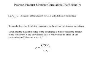
University of Warwick, Department of Sociology, 2012/13 SO 201: SSAASS (Surveys and Statistics) (Richard Lampard ) Week 5 Multiple Regression. The Correlation Coefficient (r). This shows the strength/closeness of a relationship. Age at First Childbirth. r = 0.5 (or perhaps less…).

E N D
University of Warwick, Department of Sociology, 2012/13SO 201: SSAASS (Surveys and Statistics) (Richard Lampard)Week 5Multiple Regression
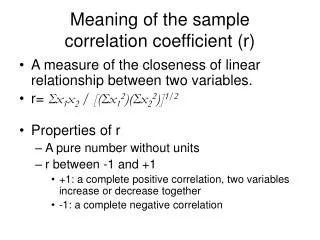
The Correlation Coefficient (r) This shows the strength/closeness of a relationship Age at First Childbirth r = 0.5 (or perhaps less…) Age at First Cohabitation
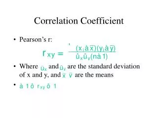
r = -1 r = + 1 r = 0
Correlation… and Regression • r measures correlation in a linear way • … and is connected to linear regression • More precisely, it is r2 (r-squared) that is of relevance • It is the ‘variation explained’ by the regression line • … and is sometimes referred to as the ‘coefficient of determination’
The arrows show the overall variation (variation from the mean of y) y Mean x
Some of the overall variation is explained by the regression line (i.e. the arrows tend to be shorter than the dashed lines, because the regression line is closer to the points than the mean line is) y Mean x
As an aside, it is worth noting that the logic of Analysis of Variance is in essence the same, the difference being that the group means, rather than a regression line, are used to ‘explain’ some of the variation (‘Between-groups’ variation). Value Line and arrow are differences from group mean and overall mean Overall mean Group 2 3 1 Analysis of Variance (ANOVA): Decomposing variance into Between-Groups and Within-Group
Outlier Length of Residence (y) B 1 ε C Age (x) 0 Regression line y = Bx + C + ε Error term (Residual) Slope Constant
Choosing the line that best explains the data • Some variation is explained by the regression line • The residuals constitute the unexplained variation • The regression line is chosen so as to minimise the sum of the squared residuals • i.e. to minimise Σε2 (Σ means ‘sum of’) • The full/specific name for this technique is Ordinary Least Squares (OLS) linear regression
Regression assumptions #1 and #2 Frequency ε 0 #1: Residuals have the usual symmetric, ‘bell-shaped’ normal distribution #2: Residuals are independent of each other
y Regression assumption #3 Homoscedasticity Spread of residuals (ε) stays consistent in size (range) as x increases x y Heteroscedasticity Spread of residuals (ε) increases as x increases (or varies in some other way) Use Weighted Least Squares x
Regression assumption #4 • Linearity! (We’ve already assumed this…) • In the case of a non-linear relationship, one may be able to use a non-linear regression equation, such as: y = B1x + B2x2 + C
Another problem: Multicollinearity • If two ‘independent variables’, x and z, are perfectly correlated (i.e. identical), it is impossible to tell what the B values corresponding to each should be • e.g. if y = 2x + C, and we add z, should we get: • y = 1.0x + 1.0z + C, or • y = 0.5x + 1.5z + C, or • y = -5001.0x + 5003.0z + C ? • The problem applies if two variables are highly (but not perfectly) correlated too…
Example of Regression(from Pole and Lampard, 2002, Ch. 9) • GHQ = (-0.69 x INCOME) + 4.94 • Is -0.69 significantly different from 0 (zero)? • A test statistic that takes account of the ‘accuracy’ of the B of -0.69 (by dividing it by its standard error) is t = -2.142 • For this value of t in this example, the significance value is p = 0.038 < 0.05 • r-squared here is (-0.321)2 = 0.103 = 10.3%
Notes on the t-value corresponding to the B • The t-value takes account of the typical amount of sampling error than can be assumed to be present, since sampling error would result in a non-zero value of B even if the population value was B=0. • This is achieved by standardising the value of B, using a standard error derived from the sum of squares of the residuals (i.e. the deviations of y from the regression line) and from a sum of squares corresponding to the variability of x (to take account of the fact that the B looks at variation in y relative to variation in x).
Why is the test statistic for the B value a t-statistic? y Consider a situation where the x variable only has two possible values, 1 unit apart. In this case the B value is equivalent to the difference between the two means for y at values 0 and 1 of x, and could thus be converted to a statistic with a t-distribution. Where there are more than two values of x, the B-value might be viewed as an average of the differences between the mean values of y for various pairs of values of x. Overall mean B The single-headed arrow and dotted line are differences from the group mean and the overall mean x 0 1
How many degrees of freedom does this t-statistic have? • In an analysis with n cases, there are n – 1 sources of variation, and hence degrees of freedom, overall. • The regression line for a single independent variable ‘uses up’ one of these sources of variation, leaving n – 2 sources of variation corresponding to the sampling error feeding into the value of B. • More generally, the number of degrees of freedom for each t-value in a multiple regression with i independent variables is n - (i + 1) • In secondary analyses of social survey data, n tends to be large, hence the t-values can often be assumed to behave like (normally distributed) z-statistics, i.e. a value of 1.96 or more will lead to a significant p-value at the 5% level,
B’s and Multivariate Regression Analysis • The impact of an independent variable on a dependent variable is B • But how and why does the value of B change when we introduce another independent variable? • If the effects of the two independent are inter-related in the sense that they interact (i.e. the effect of one depends on the value of the other), how does B vary?
Multiple Regression • GHQ = (-0.47 x INCOME) + (-1.95 x HOUSING) + 5.74 • For B = 0.47, t = -1.51 (& p = 0.139 > 0.05) • For B = -1.95, t = -2.60 (& p = 0.013 < 0.05) • The r-squared value for this regression is 0.236 (23.6%)
Comparing Bs • It does not make much sense to compare values of B, since they relate to different units (in this case pounds as compared to a distinction between types of housing). • To overcome this lack of comparability, one can look at beta (β) values, which quantify (in standard deviations) the impact of a one standard deviation change in each independent variable. In other words, they adjust the effect of each independent with reference to its standard deviation together with that of the dependent variable. • In the example here, the beta values are β=0.220 and β=0.378. Hence housing has a more substantial impact than income (per standard deviation), although this was in any case evident from the values of the t-statistics...
Dummy variables • Categorical variables can be included in regression analyses via the use of one or more dummy variables (two-category variables with values of 0 and 1). • In the case of a comparison of men and women, a dummy variable could compare men (coded 1) with women (coded 0).
Interaction effects… Women Length of residence All Men Age In this situation there is an interaction between the effects of age and of gender, so B (the slope) varies according to gender and is greater for women
Creating a variable to check for an interaction effect • We may want to see whether an effect varies according to the level of another variable. • Multiplying the values of two independent variables together, and including this third variable alongside the other two allows us to do this.
Interaction effects (continued) Women Length of residence Slope of line for women = BAGE All Men Slope of line for men = BAGE+BAGESEXD Age SEXDUMMY = 1 for men & 0 for women AGESEXD = AGE x SEXDUMMY For men AGESEXD = AGE & For women AGESEXD = 0