Download
1 / 34
340 likes | 473 Vues
5. Anisotropy decay/data analysis Anisotropy decay Energy-transfer distance distributions Time resolved spectra Excited-state reactions. This presentation has been rated XXX. Warning. The presentation contains language and images intended for a mature fluorescence audience

E N D
5. Anisotropy decay/data analysis • Anisotropy decay • Energy-transfer distance distributions • Time resolved spectra • Excited-state reactions
This presentation has been rated XXX Warning The presentation contains language and images intended for a mature fluorescence audience We are not responsible for any psychological damage that the view of the slides can cause The most offending equations will be covered and displayed only after further warning so that you can close your eyes
Basic physics concept in polarization • The probability of emission along the x (y or z) axis depends on the orientation of the transition dipole moment along a given axis. • If the orientation of the transition dipole of the molecule is changing, the measured fluorescence intensity along the different axes changes as a function of time. • Changes can be due to: • Internal conversion to different electronic states • changes in spatial orientation of the molecule • energy transfer to a fluorescence acceptor with different orientation
Anisotropy Decay • Transfer of emission from one direction of polarization to another • Two different approaches • Exchange of orientation among fixed directions • Diffusion of the orientation vector z z θ y y φ x x
Z Electric vector of exciting light Exciting light O X Y Geometry for excitation and emission polarization In this system, the exciting light is traveling along the X direction. If a polarizer is inserted in the beam, one can isolate a unique direction of the electric vector and obtain light polarized parallel to the Z axis which corresponds to the vertical laboratory axis.
Photoselection Return to equilibrium Same amount of light in the vertical and horizontal directions More light in the vertical direction Only valid for a population of molecules!
Time-resolved methodologies measure the changes of orientation as a function of time of a system. The time-domain approach is usually termed the anisotropy decay method while the frequency-domain approach is known as dynamic polarization. Both methods yield the same information. I H I V lnI time In the time-domain method the sample is illuminated by a pulse of vertically polarized light and the decay over time of both the vertical and horizontal components of the emission are recorded. The anisotropy function is then plotted versus time as illustrated here: Total intensity The decay of the anisotropy with time (rt) for a sphere is then given by:
In the case of non-spherical particles or cases wherein both “global” and “local” motions are present, the time-decay of anisotropy function is more complicated.
For example, in the case of symmetrical ellipsoids of revolution the relevant expression is: where:c1 = 1/6D2 c2 = 1/(5D2 + D1) c3 = 1/(2D2 + 4D1) where D1 and D2 are diffusion coefficients about the axes of symmetry and about either equatorial axis, respectively and: r1 = 0.1(3cos21 - 1)(3cos2 2 -1) r2 = 0.3sin2 1 sin2 2 cos r3 = 0.3sin2 1 sin2 2 (cos - sin2 ) where 1 and 2 are the angles between the absorption and emission dipoles, respectively, with the symmetry axis of the ellipsoid and is the angle formed by the projection of the two dipoles in the plane perpendicular to the symmetry axis. Resolution of the rotational rates is limited in practice to two rotational correlation times which differ by at least a factor of two.
For the case of a “local” rotation of a probe attached to a spherical particle, the general form of the anisotropy decay function is: Where 1 represents the “local” probe motion, 2 represents the “global” rotation of the macromolecule, r1 =r0(1-θ) and θ is the “cone angle” of the local motion (3cos2 of the cone aperture) In dynamic polarization measurements, the sample is illuminated with vertically polarized modulated light and the phase delay (dephasing) between the parallel and perpendicular components of the emission is measured as well as the modulation ratio of the AC contributions of these components. The relevant expressions for the case of a spherical particle are: Warning This is intended for mature audience only!!! The equation has been rated XXX by the “Fluorescence for all” International Committee and Where is the phase difference, Y the modulation ratio of the AC components, the angular modulation frequency, ro the limiting anisotropy, k the radiative rate constant (1/) and R the rotational diffusion coefficient.
At high frequency (short time) there is no dephasing because the horizontal component has not been populated yet At intermediate frequencies (when the horizontal component has been maximally populated there is large dephasing At low frequency (long time) there is no dephasing because the horizontal component and the vertical component have the same intensity
The illustration below depicts the function for the cases of spherical particles with different rotational relaxation times.
The figures here show actual results for the case of ethidium bromide free and bound to tRNA - one notes that the fast rotational motion of the free ethidium results in a shift of the “bell-shaped” curve to higher frequencies relative to the bound case. The lifetimes of free and bound ethidium bromide were approximately 1.9 ns and 26 ns respectively.
In the case of local plus global motion, the dynamic polarization curves are altered as illustrated below for the case of the single tryptophan residue in elongation factor Tu which shows a dramatic increase in its local mobility when EF-Tu is complexed with EF-Ts.
Water molecules Fluorophore electric dipole Anisotropy decay of an hindered rotator Local chisquare = 1.11873 sas 1->0 = V 0.3592718 discrete 1->0 = V 1.9862748 r0 1->0 = V 0.3960686 r-inf 1->0 = V 0.1035697 phi 1 1->0 = V 0.9904623 qshift = V 0.0087000 g_factor = F 1.0000000
Energy transfer-distance distributions Excited state k Excited state Donor-acceptor pair Simple excited state reaction No back reaction for heterotransfer All the physics is in the rate k Donor Acceptor In general, the decay is double exponential both for the donor and for the acceptor if the transfer rate is constant
The rate of transfer (kT) of excitation energy is given by: Where d is the fluorescence lifetime of the donor in the absence of acceptor, R the distance between the centers of the donor and acceptor molecules and R0 is defined by: Å Where n is the refractive index of the medium (usually between 1.2-1.4), Qd is the fluorescence quantum yield of the donor in absence of acceptor,2 is the orientation factor for the dipole-dipole interaction and J is the normalized spectral overlap integral. [() is in M-1 cm-1, is in nm and J are M-1 cm-1 (nm)4] R0 is the Förster critical distance at which 50% of the excitation energy is transferred to the acceptor and can be approximated from experiments independent of energy transfer. In principle, the distance R for a collection of molecules is variable and the orientation factor could also be variable
Analysis of the time-resolved FRET with constant rate Donor emission Acceptor emission Fluorescein-rhodamine bandpasses
General expressions for the decay Hetero-transfer; No excitation of the donor Warning This is intended for mature audience only!!! The equation has been rated XXX by the “Fluorescence for all” International Committee Intensity decay as measured at the donor bandpass Intensity decay as measured at the acceptor bandpass k1:= Γa +kt k2:= Γd ad =-Bakt bd = Bd(Γa- Γd-kt) aa = Bd(Γa- Γd)-Bdkt ba = -Ba(Γa- Γd) Γd and Γa are the decay rates of the donor and acceptor. Bd and Ba are the relative excitation of the donor and of the acceptor. The total fluorescence intensity at any given observation wavelength is given by I(t) = SASd Id(t) + SASa Ia(t) where SASd and SASa are the relative emission of the donor and of the acceptor, respectively.
If the rate kt is distributed, for example because in the population there is a distribution of possible distances, then we need to add all the possible values of the distance weighted by the proper distribution of distances Example (in the time domain) of gaussian distribution of distances (Next figure) If the distance changes during the decay (dynamic change) then the starting equation is no more valid and different equations must be used (Beechem and Hass)
FRET-decay, discrete and distance gaussian distributed Question: Is there a “significant” difference between one length and a distribution of lengths? Clearly the fit distinguishes the two cases if we ask the question: what is the width of the length distribution? Discrete Local chisquare = 1.080 Fr_ex donor 1->0 = V 0.33 Fr_em donor 1->0 = V 0.00 Tau donor 1->0 = F 5.00 Tau acceptor 1->0 = F 2.00 Distance D to A 1->0 = F 40.00 Ro (in A) 1->0 = F 40.00 Distance width 1->0 = V 0.58 Gaussian distributed Local chisquare = 1.229 Fr_ex donor 1->0 = V 0.19 Fr_em donor 1->0 = V 0.96 Tau donor 1->0 = L 5.00 Tau acceptor 1->0 = L 2.00 Distance D to A 1->0 = L 40.00 Ro (in A) 1->0 = L 40.00 Distance width 1->0 = V 26.66 gaussian discrete
FRET-decay, discrete and distance gaussian distributed Fit attempt using 2-exponential linked The fit is “poor” using sum of exponentials linked. However, the fit is good if the exponentials are not linked, but the values are unphysical Discrete distance: Local chisquare = 1.422 sas 1->0 = V 0.00 discrete 1->0 = V 5.10 sas 2->0 = V 0.99 discrete 2->0 = L 2.49 Gaussian distr distances Experiment # 2 results: Local chisquare = 4.61 sas 1->0 = V 0.53 discrete 1->0 = L 5.10 sas 2->0 = V 0.47 discrete 2->0 = L 2.49 WE NEED GLOBALS!
Time dependent spectral relaxations Solvent dipolar orientation relaxation 10-15 s 10-9 s Frank-Condon state Relaxed state Ground state Immediately after excitation Long time after excitation Equilibrium Out of Equilibrium Equilibrium
As the relaxation proceeds, the energy of the excited state decreases and the emission moves toward the red Excited state Partially relaxed state Energy is decreasing as the system relaxes Relaxed, out of equilibrium Ground state
The emission spectrum moves toward the red with time Intensity Wavelength time Wavelength Time resolved spectra What happens to the spectral width?
Time resolved spectra of TNS in a Viscous solvent and in a protein
Time resolved spectra are built by recording of individual decays at different wavelengths
Time resolved spectra can also be recoded at once using time-resolved optical multichannel analyzers
Excited-state reactions • Excited state protonation-deprotonation • Electron-transfer ionizations • Dipolar relaxations • Twisting-rotations isomerizations • Solvent cage relaxation • Quenching • Dark-states • Bleaching • FRET energy transfer • Monomer-Excimer formation
General scheme Excited state Ground state Reactions can be either sequential or branching
If the reaction rates are constant, then the solution of the dynamics of the system is a sum of exponentials. The number of exponentials is equal to the number of states If the system has two states, the decay is doubly exponential Attention: None of the decay rates correspond to the lifetime of the excited state nor to the reaction rates, but they are a combination of both
Sources on polarization and time-resolved theory and practice: Books: Molecular Fluorescence (2002) by Bernard Valeur Wiley-VCH Publishers Principles of Fluorescence Spectroscopy (1999) by Joseph Lakowicz Kluwer Academic/Plenum Publishers Edited books: Methods in Enzymology (1997) Volume 278 Fluorescence Spectroscopy (edited by L. Brand and M.L. Johnson) Methods in Enzymology (2003) Biophotonics (edited by G. Marriott and I. Parker) Topics in Fluorescence Spectroscopy: Volumes 1-6 (edited by J. Lakowicz)