Download
1 / 30
300 likes | 407 Vues
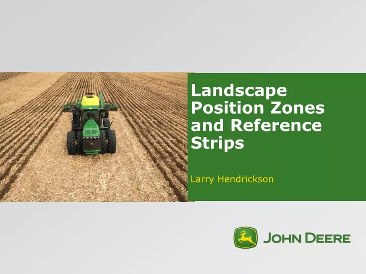
Landscape Position Zones and Reference Strips. Larry Hendrickson. 4. 1400 ft. 3. 2. 1300 ft. 1. 1200 ft. Landscape Position Zones (LSP). Extracting landscape position (LSP) from elevation data

E N D
Landscape Position Zones and Reference Strips Larry Hendrickson
4 1400 ft 3 2 1300 ft 1 1200 ft Landscape Position Zones (LSP) • Extracting landscape position (LSP) from elevation data • RTK elevation data is becoming widely available • Elevation derivatives work well for post-mortem analysis • Elevation itself isn’t usually a good means for classifying site conditions • Developed a method to extract LSP from elevation data by comparing elevation of each pixel with its neighbors | NUE 2009 Hendrickson 5 August, 2009
W Nebraska Center Pivot field W Nebraska Center Pivot field | NUE 2009 Hendrickson 5 August, 2009
LSP Zone Polygons over Corn Yield Shoulder Toeslope | NUE 2009 Hendrickson 5 August, 2009
Yield variability related to LSP—Across W NE fields Toeslope Shoulder | NUE 2009 Hendrickson 5 August, 2009
Yield variability related to LSP—Across years Toeslope Shoulder | NUE 2009 Hendrickson 5 August, 2009
Iowa field just after planting | NUE 2009 Hendrickson 5 August, 2009
Iowa field just after planting 5 4 3 2 1 | NUE 2009 Hendrickson 5 August, 2009
Iowa Corn Yield May-June Rainfall 6.1 7.8 7.6 9.4 13.2 14.9 Toeslope Shoulder Normal May-June rainfall is 9.5 inches Data from Jaynes and Kaspar | NUE 2009 Hendrickson 5 August, 2009
Iowa Soybean Yield May-June Rainfall 7.3 1.6 16.8 12.8 14.8 Toeslope Shoulder Normal May-June rainfall is 9.5 inches Data from Jaynes and Kaspar | NUE 2009 Hendrickson 5 August, 2009
Landscape Position Zones • LSP is an intuitive characteristic • Water runs downhill • Drier on shoulders, wetter on toeslopes • Often better relationship to yield than soil conductivity • In regions where topography was the primary soil forming factor | NUE 2009 Hendrickson 5 August, 2009
Role of Reference Strip in N Rate Decisions • Studies conducted by Sawyer in 2005 and 2006 • Focus on reference strip observations from these studies • Patterns observed with aerial imagery • Compare N stress outcomes with and without reference strips | NUE 2009 Hendrickson 5 August, 2009
Approach • 3 reference strips in each field with 240 or 270 #N/acre • Aerial images were taken between V10 and V14 • Calculated GNDVI from aerial images • SPAD readings were taken within 3 days of images | NUE 2009 Hendrickson 5 August, 2009
Field 1 240 N GNDVI GNDVI with upper 10% in blue | NUE 2009 Hendrickson 5 August, 2009
Field 2 | NUE 2009 Hendrickson 5 August, 2009
Field 3 | NUE 2009 Hendrickson 5 August, 2009
Imagery patterns • Considerable variability in N stress within and between reference strips • High GNDVI values were found within all fertilized (60-180N) strips, but not within zero N strips • High GNDVI values were also found in other parts of all fields examined • High GNDVI values were often impacted more by soil variability than by reference strips | NUE 2009 Hendrickson 5 August, 2009
Data Analysis • Extracted underlying GNDVI from each SPAD location • Related relative SPAD, relative GNDVI, and GNDVI relative to “best” area to yields underlying these points • Relationships across 8 studies in 2006 | NUE 2009 Hendrickson 5 August, 2009
R2 = 0.44 | NUE 2009 Hendrickson 5 August, 2009
R2 = 0.53 | NUE 2009 Hendrickson 5 August, 2009
R2 = 0.52 | NUE 2009 Hendrickson 5 August, 2009
Summary • Imagery (and presumably sensors) were more closely related to yields than SPAD values across fields • GNDVI relative to “best” areas was equivalent to using a reference strip • Reference strips were unnecessary for N decisions made after V10 in fields that had received significant rates of fertilizer earlier in the season (in Iowa) • Likely can’t extrapolate these results to other regions or earlier N applications | NUE 2009 Hendrickson 5 August, 2009
Landscape position on N requirement Shoulder Toeslope + +++ Yield Potential + +++ N Mineralization + +++ N Loss Potential Patterns of N stress observed will depend upon which factor dominates in a particular region or year | NUE 2009 Hendrickson 5 August, 2009
Estimating N Requirement • Sensor Observes Differential: • Residual N • Mineralization • Losses of soil and fertilizer N • Crop stand and growth patterns All are impacted by LSP or SC zones Early N Soil N PL Sensing | NUE 2009 Hendrickson 5 August, 2009
Estimating N Requirement • Sensor Observes Differential: • Residual N • Mineralization • Losses of soil and fertilizer N • Crop stand and growth patterns • Estimate Differential: • Losses of soil and fertilizer N • Mineralization • Crop stand and growth patterns Early N Both are often impacted by LSP or SC zones ? Soil N PL Sensing | NUE 2009 Hendrickson 5 August, 2009
Linking Soil Zones to Sensors • Soil zones are likely quite stable over time • Opportunity to re-evaluate existing sensor data obtained in large field studies by acquiring soil zones • Incorporate soil zones in future sensor evaluations • Soil zones may be useful for: • Early season applications (in fields that behave consistently across years) • Modifying algorithms to reflect differential N requirements • Directing initial pass with sensors | NUE 2009 Hendrickson 5 August, 2009
Use of zones to help select “best” areas • Imagery has advantage over sensors in that it provides data for entire field • Selection of “best” area during initial pass may offer sufficient assessment • Seems logical that “best” area in field will be in extreme soil zones (wettest/driest, darkest/lightest soils) • First pass in field should be through areas with most extreme soil conditions | NUE 2009 Hendrickson 5 August, 2009
New 2510H Applicator • Extends Sidedress Window • Clearance allows application to 30” corn • High Speed—10 mph • NH3 or UAN | NUE 2009 Hendrickson 5 August, 2009