Download
1 / 1

E N D
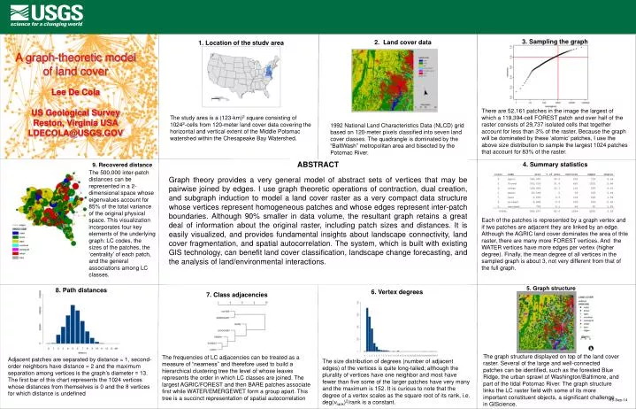
3. Sampling the graph There are 52,161 patches in the image the largest of which a 119,394-cell FOREST patch and over half of the raster consists of 29,737 isolated cells that together account for less than 3% of the raster. Because the graph will be dominated by these ‘atomic’ patches, I use the above size distribution to sample the largest 1024 patches that account for 83% of the raster. 2. Land cover data 1992 National Land Characteristics Data (NLCD) grid based on 120-meter pixels classified into seven land cover classes. The quadrangle is dominated by the “BaltWash” metropolitan area and bisected by the Potomac River. A graph-theoretic modelof land coverLee De ColaUS Geological SurveyReston, Virginia USALDECOLA@USGS.GOV 1. Location of the study area The study area is a (123-km)2 square consisting of 10242-cells from 120-meter land cover data covering the horizontal and vertical extent of the Middle Potomac watershed within the Chesapeake Bay Watershed. ABSTRACT Graph theory provides a very general model of abstract sets of vertices that may be pairwise joined by edges. I use graph theoretic operations of contraction, dual creation, and subgraph induction to model a land cover raster as a very compact data structure whose vertices represent homogeneous patches and whose edges represent inter-patch boundaries. Although 90% smaller in data volume, the resultant graph retains a great deal of information about the original raster, including patch sizes and distances. It is easily visualized, and provides fundamental insights about landscape connectivity, land cover fragmentation, and spatial autocorrelation. The system, which is built with existing GIS technology, can benefit land cover classification, landscape change forecasting, and the analysis of land/environmental interactions. 4. Summary statistics Each of the patches is represented by a graph vertex and if two patches are adjacent they are linked by an edge. Although the AGRIC land cover dominates the area of thte raster, there are many more FOREST vertices. And the WATER vertices have more edges per vertex (higher degree). Finally, the mean degree of all vertices in the sampled graph is about 3, not very different from that of the full graph. 9. Recovered distance The 500,000 inter-patch distances can be represented in a 2-dimensional space whose eigenvalues account for 85% of the total variance of the original physical space. This visualization incorporates four key elements of the underlying graph: LC codes, the sizes of the patches, the ‘centrality’ of each patch, and the general associations among LC classes. 5. Graph structure The graph structure displayed on top of the land cover raster. Several of the large and well-connected patches can be identified, such as the forested Blue Ridge, the urban sprawl of Washington/Baltimore, and part of the tidal Potomac River. The graph structure links the LC raster field with some of its more important constituent objects, a significant challenge in GIScience. 8. Path distances Adjacent patches are separated by distance = 1, second-order neighbors have distance = 2 and the maximum separation among vertices is the graph’s diameter = 13. The first bar of this chart represents the 1024 vertices whose distances from themselves is 0 and the 8 vertices for which distance is undefined 6. Vertex degrees The size distribution of degrees (number of adjacent edges) of the vertices is quite long-tailed; although the plurality of vertices have one neighbor and most have fewer than five some of the larger patches have very many and the maximum is 152. It is curious to note that the degree of a vertex scales as the square root of its rank, i.e. deg(vrank)2/rank is a constant. 7. Class adjacencies The frequencies of LC adjacencies can be treated as a measure of “nearness” and therefore used to build a hierarchical clustering tree the level of whose leaves represents the order in which LC classes are joined. The largest AGRIC/FOREST and then BARE patches associate first while WATER/EMERGEWET form a group apart. This tree is a succinct representation of spatial autocorrelation