Download
1 / 25
340 likes | 766 Vues
Optimal risky portfolio. Chapter 6. Optimal Risky Portfolio. The capital allocation decision revisited: portfolio of two risky assets Extension to the N-asset case Applications and practical issues. Idea of Diversification. Notations. P: risky portfolio F: risk-free asset

E N D
Optimal risky portfolio Chapter 6
Optimal Risky Portfolio • The capital allocation decision revisited: portfolio of two risky assets • Extension to the N-asset case • Applications and practical issues
Notations • P: risky portfolio • F: risk-free asset • y: weight allocated to P • 1-y: weight allocated to F • C: combined portfolio (P and F together) • wi: weight allocated to risky asset i in P • All the wi’s must sum up to one
Portfolio of Two Risky Assets Portfolio expected return Portfolio Variance 12 = variance of asset 1’s returns 22 = variance of asset 2’s returns Cov(r1,r2) = covariance of returns of asset 1 and asset 2
Covariance and Correlation Coefficient • Relationshipbetween the two: = Correlation coefficient of returns between assets 1 and 2 = Standard deviation of asset 1’s returns = Standard deviation of asset 2’s returns
Correlation Coefficient • Range of values for : • If = +1, the asset returns are perfectly positively correlated • If= -1, the asset returns are perfectly negatively correlated
Re-writing the variance • Re-write as: • Question: what if 1,2 = 1.0?
Example • Consider two mutual funds: • What does the line that links all the combinations of D and E look like? Depends on D,E
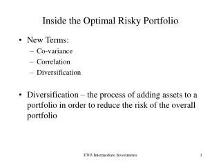
Portfolio of Two Risky Assets: Correlation Effects • The smaller the correlation, the greater the potential in risk reduction • If= +1.0, there is no reduction in risk, in the sense the standard deviation of the portfolio returns (P) is just a linear combination of D and E, i.e., no diversification benefit • Risk reduction: horizontal move toward the y axis
Minimum Variance Portfolio • Solving the minimization problem we get: • Using our example, with = 0.3: • wD= 0.82, and therefore wE = 0.18
Risk and Return of the Min. Var. Portfolio • Using the weights wD and wE, we can determine the risk-return characteristics of the minimum variance portfolio:
Extending to include a risk-free asset • Now bring back the risk-free asset, and include it in the choice of assets • What happens when you combine a different risky portfolio with the risk-free asset?
When the risk-free asset is included… • The opportunity set is again described by the (linear) CAL • The optimal risky portfolio is obtained when the slope of the CAL is maximized (i.e., when the Sharpe Ratio is maximized) • The choice of the optimal combined portfolio depends on the client’s risk attitude
The Markowitz Portfolio Selection model • Extending the concepts to n risky assets • Many possible combinations/portfolios of risky assets • Focus on portfolios that have the highest expected return for a given level of risk • Portfolios that satisfy this optimal trade-off lie on the efficient frontier • These portfolios are dominant in a mean-variance sense
Main difference between 2 risky assets and n risky assets • Two risky assets • The optimal risky portfolio is a portfolio on the curve linking all possible combinations of the two assets • n risky assets • Different possible combinations form an area, rather than a curve • Focus on the efficient frontier to determine the optimal risky portfolio