4.1 Extreme Values of Functions, p. 186

1. AP Calculus AB/BC 4.1 Extreme Values of Functions, p. 186

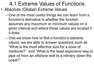
2. The mileage of a certain car can be approximated by: At what speed should you drive the car to obtain the best gas mileage? The textbook gives the following example at the start of chapter 4: Of course, this problem isn’t entirely realistic, since it is unlikely that you would have an equation like this for your car.

3. We could solve the problem graphically:

4. We could solve the problem graphically: On the TI-84, we use MATH, 7:fMax ( f(x), x, Lower Limit, Upper Limit), and the calculator finds our answer.

5. The car will get approximately 32 miles per gallon when driven at 38.6 miles per hour. We could solve the problem graphically: On the TI-84, we use MATH, 7:fMax ( f(x), x, Lower Limit, Upper Limit), and the calculator finds our answer.

6. Notice that at the top of the curve, the horizontal tangent has a slope of zero. Traditionally, this fact has been used both as an aid to graphing by hand and as a method to find maximum (and minimum) values of functions.

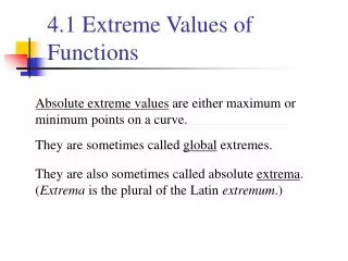
7. Even though the graphing calculator and the computer have eliminated the need to routinely use calculus to graph by hand and to find maximum and minimum values of functions, we still study the methods to increase our understanding of functions and the mathematics involved. Absolute extreme values are either maximum or minimum points on a curve. They are sometimes called global extremes. They are also sometimes called absolute extrema. (Extrema is the plural of the Latin extremum.)

8. Extreme values can be in the interior or the end points of a function. No Absolute Maximum Absolute Minimum

9. Absolute Maximum Absolute Minimum

10. Absolute Maximum No Minimum

11. No Maximum No Minimum

12. Extreme Value Theorem: If f is continuous over a closed interval, then f has a maximum and minimum value over that interval. Maximum & minimum at interior points Maximum & minimum at endpoints Maximum at interior point, minimum at endpoint

13. Local Extreme Values: A local maximum is the maximum value within some open interval. A local minimum is the minimum value within some open interval.

14. Local extremes are also called relative extremes. Absolute maximum (also local maximum) Local maximum Local minimum Local minimum Absolute minimum (also local minimum)

15. Notice that local extremes in the interior of the function occur where is zero or is undefined. Absolute maximum (also local maximum) Local maximum Local minimum

16. Local Extreme Values: If a function f has a local maximum value or a local minimum value at an interior point c of its domain, and if exists at c, then

17. Critical Point: A point in the domain of a function f at which or does not exist is a critical point of f . Note: Maximum and minimum points in the interior of a function always occur at critical points, but critical points are not always maximum or minimum values.

18. EXAMPLEFINDING ABSOLUTE EXTREMA Use analytic methods to find the extreme values of the function on the interval and where they occur. f`’(x) = 0 when x = 1, so (1, 1) is a critical point. The first derivative is undefined at x=0, so (0,0) is a critical point. Because the function is defined over a closed interval, we also must check the endpoints.

19. At: At: At: To determine if this critical point is actually a maximum or minimum, we try points on either side, without passing other critical points. Since 1<1.046 and 1<1.072, this must be at least a local minimum, and possibly a global minimum. Next, check the endpoints.

20. Absolute minimum: At: Absolute maximum: At: At: To determine if this critical point is actually a maximum or minimum, we try points on either side, without passing other critical points. Since 0<1, this must be at least a local minimum, and possibly a global minimum. Next, check the endpoints.

21. Absolute minimum (1, 1) Absolute maximum (4, 1.636)

22. 1 4 Find the derivative of the function, and determine where the derivative is zero or undefined. These are the critical points. For closed intervals, check the end points as well. 2 Find the value of the function at each critical point. 3 Find values or slopes for points between the critical points to determine if the critical points are maximums or minimums. Finding Maximums and Minimums Analytically:

23. Critical points are not always extremes! (not an extreme)

24. (not an extreme)

25. Day 2 Identify the critical points and determine the local extreme values for

27. To find critical points, we are interested in when y ' = 0. p