Tutorial 1 – Static Dipoles

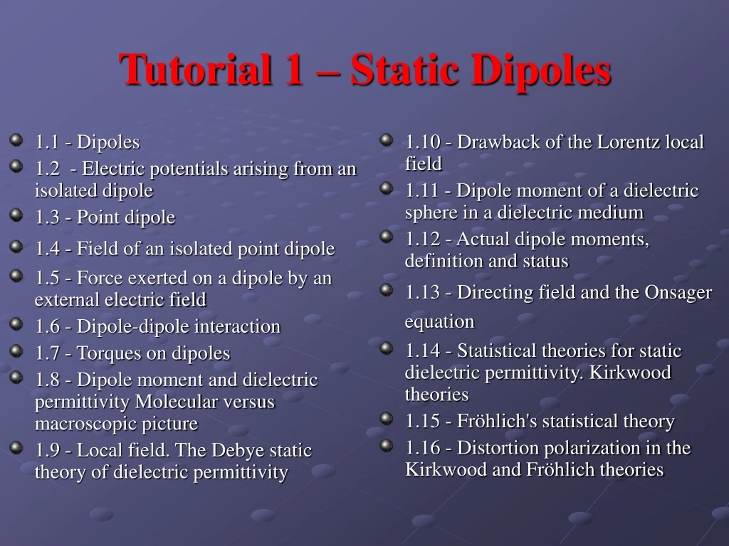
1. 1.1 - Dipoles 1.2 - Electric potentials arising from an isolated dipole 1.3 - Point dipole 1.4 - Field of an isolated point dipole 1.5 - Force exerted on a dipole by an external electric field 1.6 - Dipole-dipole interaction 1.7 - Torques on dipoles 1.8 - Dipole moment and dielectric permittivity Molecular versus macroscopic picture 1.9 - Local field. The Debye static theory of dielectric permittivity 1.10 - Drawback of the Lorentz local field 1.11 - Dipole moment of a dielectric sphere in a dielectric medium 1.12 - Actual dipole moments, definition and status 1.13 - Directing field and the Onsager equation 1.14 - Statistical theories for static dielectric permittivity. Kirkwood theories 1.15 - Fröhlich's statistical theory 1.16 - Distortion polarization in the Kirkwood and Fröhlich theories Tutorial 1 – Static Dipoles

2. These tutorials are based on the following book: Evaristo Riande, Ricardo Diaz-Calleja. Electrical Properties of Polymers. Marcel Dekker, NY, 2004

3. -q l +q 1.1 – DIPOLES. • Due to the electrical neutrality of the matter, dipoles, or multipoles are basic elements of the electric structure of the many material. • A Dipole can be defined as an entity made up by a positive charge q separated a relatively short distance l an equal negative charge. • The dipole moment is a vectorial quantity defined as • By convention, its positive direction points towards the positively charged end. • For more complicated systems, it is necessary to take into account the geometry of the molecules and interaction with other surrounding molecules.

4. Electrostatic potential at the generic point P is According with the cosine theorem, By using series expansion • 1.2. ELECTRIC POTENTIALS ARISING FROM AN ISOLATED DIPOLE z P r+ r +q d/2  r- d/2 -q

5. Where P, is the Legendre polynomials

6. Note that in equation 1.2.4, q·dcos θ = q·d · r/r (where r/r = u), and the quantity (μ = q·d is called dipolar moment. • The S.I units for dipoles is C·m, although the Debye, D, which is the dipole moment corresponding to two electronic charges separated by 0.1 nm, is a commonly used unit. Cuadripolar moment Dipolar moment

7. 1.3 - POINT DIPOLE Some times it is convenient to refers at dipoles as point dipole, that is: a point in the space, with moment and direction μ

8. 1.4 - FIELD OF AN ISOLATED POINT DIPOLE • The dipole potential can be written as • The electric field is • After some calculations, one obtains • The field, expressed in matrix is

9. 1.5 - FORCE EXERTED ON A DIPOLE BY ANEXTERNAL ELECTRIC FIELD • Consider a dipole located in an external electric field Eo. The total force acting on the dipole is the sum of the forces acting on each charge, that is (1.5.1) • If d is very small in comparison with r, the first term on the right-hand side of Eq.(1.5.1) can be expanded into a Taylor series around r, giving (1.5.2) • substituting Eq ( 1.5.2) into Eq ( 1.5.1) and neglecting terms of order d2 and higher, we obtain (1.5.3)

10. The electrical force can also be derived from the potential electrical energy U, noting that (1.5.5) • For a single charge q, the ratio of Eq (1.5.5) to q gives Eo= - Φ. By comparing Eqs (1.5.3) and (1.5.5), the potential for a single dipole is given by (1.5.6)

11. For an arbitrary external electric field, Eq (1 5.3) can be written in terms of the components as

12. 1.6. DIPOLE - DIPOLE INTERACTION • The energy of a system formed by two dipoles µ1 and µ2is the work done on one of these dipoles placed in the field of the other dipole. According to Eq.(1.4.3), the energy is: • the force exerted on one of these dipoles owing to the field produced by the other is

13. Special cases If µ1=µ2= µ, the mutual force will be For parallel dipoles (µ1=µ2) perpendicular to r For antiparallel dipoles (µ1=-µ2) perpendicular to r • Finally, for perpendicular dipoles that are both also perpendicular to r

14. -q +q 1.7. TORQUES ON DIPOLES • The total torque is • Neglecting the term of high order and considering the dipole definition, Fo Eo d/2 d/2 Fo

15. The torque is null when µ and Eo are parallel. As a consequence of the torque, the dipole tends to reorient along the field, even in the presence of a uniform field. This is a consequence of the not cancellation of the torque of two opposite non collinear forces. The work of reorientation from a position perpendicular to the field to another forming an angle θis given by

16. 1.8. DIPOLE MOMENT AND DIELECTRICPERMITTIVITY. MOLECULAR VERSUSMACROSCOPIC PICTURE • In real situationscontinuous medium enormous number of elementary dipoles. • Dipolar substances contain permanent dipoles arising from the asymmetrical locating of electric charges in the matter. • Under an electric field, these dipoles tend to orient as a result of the action of torques, • The macroscopic result is the orientation polarization of the material

17. The effect of the applied electric field is also to induce a new types of polarization • by distortion of the electronic clouds (electronic polarization) • and the nucleus (atomic polarization) of the atomic structure Time scale to reach equilibrium 10-10~10-12 s. Under an applied field of frequency 1010~1012 Hz, the orientation polarization scarcely contributes to the total polarization. However, this contribution increases when the frequency diminishes (time increases), and this is the essential feature of the dielectric dispersion. For a static case, the fieldE acting on a dipole is, in general, different from the applied field Eo. The average moment for an isotropic material can be written as • where αistotal polarizability (includes the electronic, αe, the atomic, αa, and the orientational, αo, contributions)

18. Equation (1.8.1)is strictly true only if E is small. This means : • no saturation effects • relationship between the induced moment and theelectric field is of the linear type. The total polarization ofN1dipolar molecules per unit volume, each of them having an average moment m, is where N is the total number of molecules. The average field caused by the induced dipoles of the dielectric placed between two parallel plates is given by The mean electric field (Ez) must be added to the field arising from the charge densities in the plates.

19. This field is given by (D electric displacement) • The dielectric susceptibility is defined as εris the relative permittivity and εo (= 8,854x 10-l2C2kg-1m-3s2) is the permittivity ofthe free space. In c.g.s. units, εo= 1 and εr= ε

20. 1.9. LOCAL FIELD. THE DEBYE STATIC THEORY OF DIELECTRIC PERMITTIVITY • Until now the dipolar structure of the dielectric was considered, but the electric field acting on the dipoles was not determined. • For the evaluation of the static dielectric permittivity in terms of the dipole moment μ of the molecules of the dielectric require the determination of the LOCAL FIELD acting upon the molecules and the ratio of the dipole moment of the molecule and either the polarizability αo or the average moment m. • The concept of INTERNAL FIELD has received considerable attention because it relates macroscopic properties to molecular ones. The problem involved in the determination of the field acting on a single dipole in the dielectric is its dependence on the polarization of the neighboring molecules.

21. The first approach to the analysis in this problem is due to Lorentz. • The basic idea is to consider a a spherical zone containing the dipole under study, immersed in the dielectric. • The sphere is small in comparison with the dimension of the condenser, but large compared with the molecular dimensions. • We treat the properties of the sphere at the microscopic level as containing many molecules, but the material outside of the sphere is considered a continuum. • The field acting at the center of the sphere where the dipole is placed arises from the field due to • (1) the charges on the condenser plates • (2) the polarization charges on the spherical surface, and • (3) the molecular dipoles in the spherical region.

22. d - - - - E - - + + + + + + The field due to the polarization charges on the spherical surface, Esp, can be calculated by considering an element of the spherical surface defined by the angles θ and θ+dθ. The area of this elementary surface is: 2πr2sin θdθ. The density of charge on this element is given by P·cosθ, and the angles between this polarization and the elementary surface is θ. Integrating over all values of angle formed by the direction of the field with the normal vector to spherical surface at each point and dividing by the surface of the sphere we obtain 

23. The polarization was previously defined(1.8.6) as: • Therefore, the total field will be • This is the Lorentz field.

24. By combining Eqs (1.9.2),(1.9.3), and (1.8.1), the following equation relating the permittivity and the total polarizability is obtained: Here, the assumption that m=μ (dilute systems) is made. If the material has molecular weight M, and density ρ, then N1=ρNAM, where NA is the Avogadro’s number, in this case the equation 1.9.4 becomes: This is the Claussius – Mossotti equation valid for nonpolar gases at low pressure. This expression is also valid for high frequency limit. The remaining problem to be solved is the calculation of the dipolar contribution to the polarizability.

25. The first solution to this problem for the static case was proposed by Debye. • In absence of structure, the potential energy of a dipole of μ is given by: • In this case, Ei is the internal field, instead of the external applied field Eo, because Ei is the field acting upon the dipole. • If a Boltzmann distribution for the orientation of the dipoles axis is assumed, the probability to find a dipole within an elementary solid angle dΩ is given by • The average value of the dipole moment in the direction of the field is

26. After integration by parts Where L(y)=coth y – y-1denotes the Langevin function given by For y<<1, the Langevin function is approximately L(y)y/3, and the orientational polarization is given by If the distortional polarizability dis added, the total polarization is

27. By substituting Eq (1.9.3) into Eq (1.9.12) and taking into account Eq(1.9.2), one obtain Debye equation for the static permittivity

28. At very high frequencies, dipoles do not have time for reorientation and the dipolar contribution to permittivity is negligible. Then, Where d=∞. Since the infinite frequency permittivity is equal to the square of the refraction index, n, Eq (1.9.15) becomes Lorentz-Lorenz equation Note that equation 1.9.16, can be rewritten as where =1/, is the specific volume, and C=4NA/3M. By plotting the C(n2+2)/(n2+1) vs T-1, the isobaric dilatation coefficient can be obtained, and, eventually, the glass transition temperature could be estimated. Note that from the temperature dependence of the index of refraction of glassy systems, physical aging and related phenomena could be analyzed.

29. 1.10. DRAWBACK OF THE LORENTZ LOCAL FIELD For highly polar substances, the dipolar contribution to the polarizability is clearly dominant over the distorortional one. From previous equations and substituting o=2/3kT, the susceptibility becomes infinite at a temperature given by This temperature , is called Curie temperature. This equation suggest that at temperature , spontaneous polarization should occur and the material should become ferroelectric, even in absence of an electric field.

30. Ferro-electricity is uncommon in nature, and predictions made by Eq (1.10.1) are not experimentally supported. • The failure of this theory arises from considering null the contribution to the local field of the dipoles in the cavity. • This fact emphasizes the inadequacy of the Lorentz field in a dipolar dielectric and leaves open the question of the internal field in the cavity.

31. 1.11. DIPOLE MOMENT OF A DIELECTRIC SPHERE IN A DIELECTRIC MEDIUM • Claussius-Mossotti equation represent the first attempt to relate a macroscopic quantity, the dielectric permittivity, to the microscopic polarizability of the substances. • The equation only is valid for the displacement polarization. • To solve the same problem for the orientational polarizability is much more complicated. • The starting point of the solution to the problem of the local field in the context of the theory of the orientational polarization is to consider a spherical cavity of radius a and relative permittivity 1, that contains at the center a rigid dipolar molecule with permanent dipole.

32. The radius of the cavity is obtained form the relation • Where N is the number of molecules in a volume V. In many cases a can be considered as the “molecular radius”. • This cavity is assumed to be surrounded by a macroscopic spherical shell of radius b>>a, and the relative permittivity 2. • The ensemble is embedded in a continuum medium of relative permittivity 3.

33. According to Onsager, the internal field in the cavity has two components: 1 – The cavity field, G, (the field produced in the empty cavity by the external field.) 2 - The reaction field, R (the field produced in the cavity by the polarization induced by the surrounding dipoles). Dielectric or conducting shells are technologically important, and biological cells are also examples of layered spherical structures.

34. The general solution of the Laplace equation (2ф=0), in spherical coordinates and for the case of axial symmetry, is Where the i subscript refers to each one of the three zones under consideration. For our particular geometry, the following boundary condition hold These conditions arise from the fact that the only charges existing in the cavity contributing to ф1 belong to the dipole. The contribution of the external field to ф3, for r>>>b is Eor·cosθ.

35. Owing the boundary conditions, only the first term of the polynomial (cos θ) appears in the Eq. 1.11.2, so that series of spherical harmonics is greatly simplified. Consequently the potentials are Solving the system of equation 1.11.3 and 1.11.4, the resulting potentials are: (1.11.5)

37. Special Cases: 1 – Empty cavity, in this case 1=1, and all the terms in Eq 1.11.7 containing  as a factor vanish. The resulting potential are given by 2 – Dipole point in the center of the empty cavity. Absence of external field. In this case, again 1=1, and the terms containig Eo vanish. The potentials are given by

38. It could be also useful to consider the inner cavity in a continuum, that is, without spherical shell. In this case, 2=3, and consequently G32=1, and R32=0. Thus the Equations 1.11.8 and 1.11.9 become respectively These results indicate that the field in an empty cavity embedded in a dielectric medium with permittivity 2 is On the other hand, dipoles induce on the surface of the spherical cavity (even in absence of external field) an electric field opposing that of the dipole himself, called the reaction field,

39. 3 – Finally, for 1=3=1, Eq (1.11.7) leads to

40. 1.12. ACTUAL DIPOLE MOMENTS, DEFINITION AND STATUS The potential of a rigid non-polarizable dipole in a medium of relative permittivity 1 is given by (e subscript means external) Usually, dipoles are associated to molecules having an electronic cloud that shields them. Thus let us consider a dipole  in the center of a sphere representing the molecule. The electronic polarizability of the sphere gives rise at a macroscopic level, to an instantaneous permittivity . In this case, the potential is given by

41. By identifying the potentials in Eqs. (1.12.1) and (1.12.2), one find Where eis called the external moment of a molecule in a medium with relative permittivity 1. The dipole molecule in vacuum will be However, the total moment of the molecule, also called the internal moment, is the vector sum of its vacuum value and the value induced in it by the reaction field, that is Which can be written as If the polarizability  is known,

42. Then, one obtain Internal dipole moment Note that it expression is independent of the size of the spherical specimen. So, if a very large sphere containing a dipole with internal moment i, in a infinite dielectric medium of relative permittivity 1 is considered, the dipole moment of the large sphere is also, i. For =1 , the following expression holds Note that the factor appearing in Eq (1.12.10), also appear in Eq. (1.11.12c) The internal moment can be also written as The internal moment can also be calculated as the geometric sum of the external moment of the dipole and the moment of a sphere with the same permittivity as the medium surrounding the dipole. In this conditions

43. Although this integral can be obtained by a simple electrostatic calculation, it can also be determined by comparing Eqs (1.12.11) and (1.12.12), that is

45. 1.13 DIRECTING FIELD AND THE ONSAGER EQUATION previously, the internal dipole moment has been calculated in absence of an external field. When this force field is applied, it is necessary to take into account this effect. In fact the total field in the cavity is now the superposition of the cavity field G with the field due to the dipole From which Where  is given by Eq. (1.12.8) The mean value of the dipole moment parallel to the external field is calculated form the Boltzmann distribution for the orientational polarization given by Eq. (1.9.6) and (1.9.7). However, the energy of the dipole is calculated from the torque acting on the molecule, which according to Eq (1.13.1) is given by

46. From Eq. (1.13.2) into Eq. (1.13.3) From Eq. (1.7.3) it follows that (U=∫d) Equations (1.9.8) and (1.13.5) lead to By substituting this equation into Eq. (1.13.2) On the other hand, the polarization per unit of volume is

47. Substitution of the Eq. (1.13.7) into the Eq. (1.13.8) gives Where the quantity Is called DIRECTING FIELD, Ed. The directing field is calculated as the sum of cavity field and the reaction field caused by a fictive dipole Ed. Note: Directing field must be not confused with the internal field Ei. Ei= Ed+R According to these results, Eq. (1.13.9) can be written as

48. Rearrangement of Eq (1.13.9), taking into account Eq. (1.12.8), gives the Onsager expression It is interesting to compare the Debye results (Eq 1.9.11) and the Onsager theories. The Lorentz local field (Eq. 1.9.3) change Eq.(1.9.11) to Comparison of Eqs. (1.13.13) and (1.13.11), leads to the conclusion that the Onsager theory takes for the internal and directing fields more accurate values that older theories in which Lorentz field is used. Note that, after some rearrangements, the Onsager equation can be written as

49. It is clear that Onsager equation does not predict ferro-electricity as the Debye equation does. In fact, the cavity field tends to 3Eo/2, when ε1 tends to infinite. Onsager takes into account the field inside the spherical cavity that caused by molecular dipoles, which is neglected in the Debye theory. However, following the Boltzmann-Langevin methodology, the Onsager theory neglects dipole – dipole interactions, or equivalently, local directional forces between molecular dipoles are ignored. The range of applicability of the Onsager equation is wider than that of the Debye equation. For example, it is useful to describe the dielectric behavior on non-interacting dipolar fluids, but in general this is not valid for condensed matter.

50. 1.14. STATISTICAL THEORIES FOR STATIC DIELECTRIC PERMITTIVITY.KIRKWOOD’S THEORY • Onsager treatment of the cavity differs from Lorentz’s because the cavity is assumed to be filled with a dielectric material having a macroscopic dielectric permittivity. • Also Onsager studies the dipolar reorientation polarizability on statistical grounds as Debye does. • However, the use of macroscopic argument to analyze the dielectric problem in the cavity prevents the consideration of local effects which are important in condensed matter. • This situation led Kirkwood first, and Fröhlich later on the develop a fully statistical argument to determine the short – range dipole – dipole interaction.