Download

1 / 19
190 likes | 305 Vues
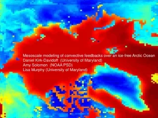
Mesoscale modeling of convective feedbacks over an ice-free Arctic Ocean Daniel Kirk-Davidoff (University of Maryland) Amy Solomon (NOAA PSD) Lisa Murphy (University of Maryland).

E N D
Mesoscale modeling of convective feedbacks over an ice-free Arctic Ocean Daniel Kirk-Davidoff (University of Maryland) Amy Solomon (NOAA PSD) Lisa Murphy (University of Maryland)
High polar temperatures during PETM and Eocene Optimum remain difficult to simulate in GCMs with plausible carbon dioxide concentrations and tropical temperatures • This suggests that there are feedback mechanisms that are not being captured by GCMs. What could they be missing? • Hurricanes (Emanuel & Korty’s ideas) • Polar Stratospheric Clouds (Sloan & Pollard, Kirk-Davidoff et al.) • Cloud feedbacks (Kump & Pollard) • Convective feedbacks (Abbott & Tzipperman) • Here we test whether the use of higher resolution and better treatment of cloud water and cloud ice transport can significantly change the response of outgoing longwave radiation to surface temperature changes.
Procedure: We ran NCAR’s CAM3.0 at T42 resolution (about 2.8° x 2.8°) with a fixed SST distribution. SST’s are modified from the current climate so that temperatures in the tropics are held constant, but temperatures at high latitudes do not fall below Tp . We ran five experiments for two years each, with Tp = 10, 11, 12 13, 14, 15 °C. Output from these runs was then used to force the Weather Research and Forecast Model (WRF). WRF was run at a resolution of 50 km, using two different convection parameterizations, using a square domain centered at the north pole, and extending south to about 65° N. We also performed a run of WRF with a much smaller domain, and a resolution of 5 km, and no convection code. Each WRF run was repeated using the 10, 12, and 15 °C CAM run output (and the corresponding SST distributions) for boundary forcing.
Tp = 15°C CAM results Tp = 10°C
Tp = 15°C CAM results: OLR Tp = 10°C
Conclusions • WRF is much more resistant to high latitude warmth than CAM • OLR is higher at each SST • d(OLR)/dT is larger • The reason for this is that WRF has lower high cloud concentrations, and these respond less strongly to SST changes. • There are big differences in water vapor and cloud ice feedbacks as well, but these are of secondary importance in setting the overall radiative feedback to surface temperature • Going to high resolution in the polar region appears to make Eocene polar warmth harder, rather than easier to explain.