Download
1 / 55
610 likes | 895 Vues
+ D x. Matching. Influence. 5. SOURCES OF ERRORS. 5.2. Noise types. 5.2. Noise types. In order to reduce errors, the measurement object and the measurement system should be matched not only in terms of output and input impedances, but also in terms of noise. x. Measurement Object.

E N D
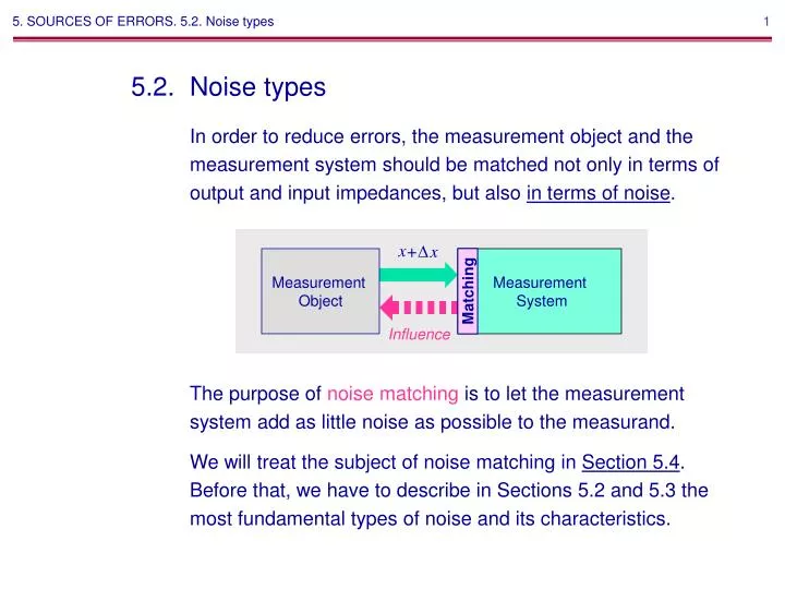
+Dx Matching Influence 5. SOURCES OF ERRORS. 5.2. Noise types 5.2. Noise types In order to reduce errors, the measurement object and the measurement system should be matched not only in terms of output and input impedances, but also in terms of noise. x Measurement Object Measurement System The purpose of noise matching is to let the measurement system add as little noise as possible to the measurand. We will treat the subject of noise matching in Section 5.4. Before that, we have to describe in Sections 5.2 and 5.3 the most fundamental types of noise and its characteristics.
MEASUREMENT THEORY FUNDAMENTALS. Contents 5. Sources of errors 5.1. Impedance matching 5.4.1. Anenergetic matching 5.4.2. Energic matching 5.4.3. Non-reflective matching 5.4.4. To match or not to match? 5.2. Noise types 5.2.1. Thermal noise 5.2.2. Shot noise 5.2.3. 1/f noise 5.3. Noise characteristics 5.3.1. Signal-to-noise ratio,SNR 5.3.2. Noise factor, F, and noise figure,NF 5.3.3. Calculating SNR and input noise voltage from NF 5.3.4. Vn-Innoise model 5.4. Noise matching 5.4.1. Optimum source resistance 5.4.2. Methods for the increasing of SNR 5.4.3. SNR of cascaded noisy amplifiers
5. SOURCES OF ERRORS. 5.2. Noise types. 5.2.1. Thermal noise 5.2.1. Thermal noise Thermal noise is observed in any system having thermal losses and is caused by thermal agitation of charge carriers. Thermal noise is also called Johnson-Nyquist noise. (Johnson, Nyquist: 1928, Schottky: 1918). An example of thermal noise can be thermal noise in resistors. Reference: [1]
vn(t) 2s 6s Vn f(vn) Normal distribution according to the central limit theorem 2R(t) en2 White (uncorrelated) noise t f 0 0 5. SOURCES OF ERRORS. 5.2. Noise types. 5.2.1. Thermal noise Example: Resistor thermal noise vn(t) T 0 R V t
C enC T 5. SOURCES OF ERRORS. 5.2. Noise types. 5.2.1. Thermal noise A. Noise description based on the principles of thermodynamics and statistical mechanics (Nyquist, 1828) To calculate the thermal noise power density, enR2( f ), of a resistor, which is in thermal equilibrium with its surrounding, we temporarily connect a capacitor to the resistor. Real resistor R Ideal, noiseless resistor enR T Noise source From the point of view of thermodynamics, the resistor and the capacitor interchange energy:
mv2 2 5. SOURCES OF ERRORS. 5.2. Noise types. 5.2.1. Thermal noise Illustration: The law of the equipartition of energy z Each particle has three degrees of freedom mivi 2 2 y x mi vi 2 2 mv2 2 kT 2 In thermal equilibrium: = =3
CV2 2 CVC 2 2 kT 2 In thermal equilibrium: = 5. SOURCES OF ERRORS. 5.2. Noise types. 5.2.1. Thermal noise Illustration: Resistor thermal noise pumps energy into the capacitor z Each particle (mechanical equivalents of electrons in the resistor) has three degrees of freedom The particle (a mechanical equivalent of the capacitor) has a single degree of freedom mivi 2 2 y x
C enC T CVC 2 2 kT 2 In thermal equilibrium: = 5. SOURCES OF ERRORS. 5.2. Noise types. 5.2.1. Thermal noise enC ( f ) enR ( f ) H( f ) = Real resistor R Ideal, noiseless resistor enR T Noise source Since the obtained dynamic first-order circuit has a single degree of freedom, its average energy is kT/2. This energy will be stored in the capacitor:
According to the Wiener–Khinchin theorem (1934), Einstein (1914), CsnC2 kT kT CvnC(t)2 = = snC2 = . 2 2 C 2 enR 2(f)H(j2pf)2ej2pf tdf snC2 = RnC (0) = 0 enR2(f) 1 = enR2(f) df = 4RC 1+ (2pfRC)2 0 Power spectral density of resistor noise: enR2(f)= 4kTR [V2/Hz]. 5. SOURCES OF ERRORS. 5.2. Noise types. 5.2.1. Thermal noise CVC 2 2 = kT = . C
enR P(f)2 enR(f)2 1 R = 50 W, C= 0.04 fF 0.8 0.6 0.4 0.2 f 1 GHz 10 GHz 100 GHz 1 THz 10 THz 100 THz SHF EHF IR R 5. SOURCES OF ERRORS. 5.2. Noise types. 5.2.1. Thermal noise B. Noise description based on Planck’s law for blackbody radiation (Nyquist, 1828) hf ehf /kT-1 enR P2(f)= 4R [V2/Hz]. A comparison between the two Nyquist equations:
eqn (f)2 enR (f)2 8 6 Quantum noise 4 2 0 f SHF EHF IR R 1 GHz 10 GHz 100 GHz 1 THz 10 THz 100 THz 5. SOURCES OF ERRORS. 5.2. Noise types. 5.2.1. Thermal noise C. Noise description based on quantum mechanics (Callen and Welton, 1951) The Nyquist equation was extended to a general class of dissipative systems other than merely electrical systems: hf ehf / kT-1 hf 2 eqn2(f)= 4R + [V2/Hz] Zero-point energyf(T)
5. SOURCES OF ERRORS. 5.2. Noise types. 5.2.1. Thermal noise The ratio of the temperature dependent and temperature independent parts of the Callen-Welton equation shows that at 0 K and f 0 there still exists some noise compared to the Nyquist noise level at T0= 290 K (standard temperature: kT0= 4.0010-21) 2 ehf / kTstd-1 10Log [dB] 100 103 106 109 f, Hz 0 -20 Remnant noise at 0 K, dB -40 -60 -80 -100 -120
Equal areas Equal areas 0 5. SOURCES OF ERRORS. 5.2. Noise types. 5.2.1. Thermal noise D. Equivalent noise bandwidth, B An equivalent noise bandwidth,B,is defined as the bandwidth of an equivalent-gain ideal rectangular filter that would pass as much power of white noise as the filter in question: IA(f)I2 IAmax I2 Bdf . IA(f)I2 IAmax I2 B B Lowpass Bandpass 1 0.5 f 0 linear scale Df Df
=en in2H(f)2 df 0 1 1 + (f / fc )2 = en in2 df = en in20.5p fc Vn o 2= en in2B 0 5. SOURCES OF ERRORS. 5.2. Noise types. 5.2.1. Thermal noise Example: Equivalent noise bandwidth of an RC filter R en o(f) Vn o 2=en o2(f)df 0 C enR 1 2pRC fc = = D f3dB
en o2 en o2 B=0.5pfc = 1.57fc en in2 en in2 Equal areas Equal areas 0.5 fc B 1 0.5 0.1 fc f /fc 0.01 0.1 1 10 100 5. SOURCES OF ERRORS. 5.2. Noise types. 5.2.1. Thermal noise Example: Equivalent noise bandwidth of an RC filter R en o 1 C en in f /fc 1 2pRC fc = = D f3dB 1 0 2 4 6 8 10
Butterworth filters: 1 1+ ( f /fc )2n H( f )2 = 5. SOURCES OF ERRORS. 5.2. Noise types. 5.2.1. Thermal noise Example: Equivalent noise bandwidth of higher-order filters First-order RC low-pass filterB= 1.57fc. Two first-order independent stages B= 1.22fc. • second order B= 1.11fc. • third order B= 1.05fc. • fourth order B= 1.025fc.
At room temperature: en = 0.13R[nV/Hz]. 5. SOURCES OF ERRORS. 5.2. Noise types. 5.2.1. Thermal noise Amplitude spectral density of noise, rms/Hz0.5: en = 4kTR[V/Hz]. Noise voltage, rms: Vn = 4kTRB[V].
Examples: Vn= 4kT1MW1MHz = 128 mV Vn= 4kT1kW1Hz = 4 nV Vn= 4kT50W1Hz = 0.9 nV 5. SOURCES OF ERRORS. 5.2. Noise types. 5.2.1. Thermal noise
5. SOURCES OF ERRORS. 5.2. Noise types. 5.2.1. Thermal noise 1) First-order filtering of the Gaussian white noise. E. Normalization of the noise pdf by dynamic networks Input noise pdf Input and output noise spectra Output noise pdf Input and output noise vs. time
5. SOURCES OF ERRORS. 5.2. Noise types. 5.2.1. Thermal noise 1) First-order filtering of the Gaussian white noise. Input noise pdf Input noise autocorrelation Output noise pdf Output noise autocorrelation
5. SOURCES OF ERRORS. 5.2. Noise types. 5.2.1. Thermal noise 2) First-order filtering of the uniform white noise. Input noise pdf Input and output noise spectra Output noise pdf Input and output noise vs. time
5. SOURCES OF ERRORS. 5.2. Noise types. 5.2.1. Thermal noise 2) First-order filtering of the uniform white noise. Input noise pdf Input noise autocorrelation Output noise pdf Output noise autocorrelation
5. SOURCES OF ERRORS. 5.2. Noise types. 5.2.1. Thermal noise F. Noise temperature, Tn Different units can be chosen to describe the spectral density of noise: mean square voltage (for the equivalent Thévenin noise source), mean square current (for the equivalent Norton noise source), and available power. R en2 = 4kTR[V2/Hz], en(f) in(f) R in2 = 4kT/R[A2/Hz], R na(f) en2 na= kT[W/Hz]. en(f) 4R
5. SOURCES OF ERRORS. 5.2. Noise types. 5.2.1. Thermal noise Any thermal noise source has available power spectral density na( f ) = kT ,where T is defined as the noise temperature, T Tn. It is a common practice to characterize other, nonthermal sources of noise, having available power that is unrelated to a physical temperature, in terms of an equivalent noise temperature Tn: na(f) na( f ) en(f) Tn ( f ) . k Nonthermal sources of noise Then, given a source's noise temperature Tn, na( f ) kTn ( f ) .
5. SOURCES OF ERRORS. 5.2. Noise types. 5.2.1. Thermal noise Example A: Noise temperatures of nonthermal noise sources 1. Environmental noise: Tn(1 MHz) can be as great as 3108 K. 2. Antenna noise temperature: T l vn2(f)= 320p2(l/l)2kT [WJ/Hz]= 4 kTa RS [V2/Hz] l << l RS = 80p2(l/l)2[W]is the radiation resistance. Reference: S. I. Baskakov.
5. SOURCES OF ERRORS. 5.2. Noise types. 5.2.1. Thermal noise Example B: Antenna noise temperature, Ta (sky contribution only) 104 Galactic noise limit TG 100 l2.4 103 O2 300 H2O Antenna noise temperature, Ta (K) 102 101 Quantum noise limit TQ = hf/k 100 100 101 102 103 104 105 106 107 108 109 Frequency, MHz S. Okwit, “An historical view of the evolution of low-noise concepts and techniques,” IEEE Trans. MT&T, vol. 32, pp. 1068-1082, 1984.
5. SOURCES OF ERRORS. 5.2. Noise types. 5.2.1. Thermal noise Example C: Noise performance of any antenna/receiving system, Top Antenna Receiver Ta RS G vS l Ta +Te Noiseless Tais the antenna noise temperature, K, Teis the effective input receiver temperature, K, Top= Ta+Teis the operating noise temperature, K. Compare: a 75 K receiver versus a 80 K receiver, vis-à-vis a 0.999-dBreceiver versus a 1.058-dB receiver. S. Okwit, “An historical view of the evolution of low-noise concepts and techniques,” IEEE Trans. MT&T, vol. 32, pp. 1068-1082, 1984.
5. SOURCES OF ERRORS. 5.2. Noise types. 5.2.1. Thermal noise G. Thermal noise in capacitors and inductors We will show in this section that in thermal equilibriumany system that dissipates power generates thermal noise; and vice versa, any system that does not dissipate power does not generate thermal noise. For example, ideal capacitors and inductors do not dissipate power and then do not generate thermal noise. To prove the above, we will show that the following circuit can only be in thermal equilibrium if enC = 0. R C enR enC T T Reference: [2], pp. 230-231
f > 0 f > 0 5. SOURCES OF ERRORS. 5.2. Noise types. 5.2.1. Thermal noise PRC R C PCR enR enC T T In thermal equilibrium, the average power that the resistor delivers to the capacitor, PRC, must equal the average power that the capacitor delivers to the resistor, PCR. Otherwise, the temperature of one component increases and the temperature of the other component decreases. PRC is zero, since the capacitor cannot dissipate power. Hence, PCR should also be zero: PCR= [enC(f)HCR(f)]2/R = 0, where HCR(f)= R/(1/j2pf+R). Since HCR(f) 0, enC (f)= 0. Reference: [2], p. 230
=enR2H(f)2 df 0 VnC 2 1 2pRC = 4kTR 0.5p 5. SOURCES OF ERRORS. 5.2. Noise types. 5.2.1. Thermal noise H. Noise power at a capacitor Ideal capacitors and inductors do not generate any thermal noise. However, they doaccumulate noise generated by other sources. For example, the noise power at a capacitor that is connected to an arbitrary resistor value equals kT/C: R C = 4kTRB VnC enR T kT C VnC 2= Reference: [5], p. 202
5. SOURCES OF ERRORS. 5.2. Noise types. 5.2.1. Thermal noise The rms voltage VnC across the capacitor does not depend on the value of the resistor because small resistances have less noise spectral density but result in a wide bandwidth, compared to large resistances, which have reduced bandwidth but larger noise spectral density. To lower the rms noise level across a capacitors, either capacitor value should be increased or temperature should be decreased. R kT C C VnC 2= VnC enR T Reference: [5], p. 203
www.discountcutlery.net 5. SOURCES OF ERRORS. 5.2. Noise types. 5.2.2. Shot noise 5.2.2. Shot noise D Shot noise (Schottky, 1918) results from the fact that the current is not acontinuous flow but the sum of discrete pulses, each corresponding to the transfer of an electron through the conductor. Its spectral density is proportional to the average current and is characterized by a white noise spectrum up to a certain frequency, which is related to the time taken for an electron to travel through the conductor. In contrast to thermal noise, shot noise cannot be reduced by lowering the temperature. I ii Reference: Physics World, August 1996, page 22
5. SOURCES OF ERRORS. 5.2. Noise types. 5.2.2. Shot noise Illustration: Shot noise in a diode D i I t Reference: [1]
I 5. SOURCES OF ERRORS. 5.2. Noise types. 5.2.2. Shot noise Illustration: Shot noise in a diode D i I t Reference: [1]
5. SOURCES OF ERRORS. 5.2. Noise types. 5.2.2. Shot noise A. Statistical description of shot noise We start from defining n as the average number of electrons passing the p-n junction of a diode during one second, hence, the average electron current I = qn. We assume that the probability of passing two or more electrons simultaneously is negligibly small,P>1(dt) = 0. This allows us to define the probability that an electron passes the junction in the time interval dt = (t, t+dt) as P1(dt) =ndt (dt is approaching the timetaken for an electron to travel over the junction, < 1 ns). vDt
5. SOURCES OF ERRORS. 5.2. Noise types. 5.2.2. Shot noise Next, we derive the probability that no electrons pass the junction in the time interval (0, t+dt): P0(t+dt) = P0(t)P0(dt) = P0(t)[1-P1(dt)] = P0(t) -P0(t) ndt. This yields: with the obvious initiate state P0(0) = 1. dP0 dt = -nP0
5. SOURCES OF ERRORS. 5.2. Noise types. 5.2.2. Shot noise The probability that an electron passes the junction in the time interval (0, t+dt) P1(t+dt) = P1(t) P0(dt) + P0(t) P1(dt) = P1(t) (1-ndt) + P0(t) ndt . This yields with the obvious initiate state P1(0) = 0. dP1 dt = -nP1 +nP0
5. SOURCES OF ERRORS. 5.2. Noise types. 5.2.2. Shot noise In the same way, one can obtain the probability of passing the junction N electrons: dPN dt = -nPN+nPN -1 . PN(0) = 0 By substitution, one can verify that (nt)N N! PN (t) = e- n t, which corresponds to the Poisson probability distribution.
(nt)N N! PN(t) =e- nt 5. SOURCES OF ERRORS. 5.2. Noise types. 5.2.2. Shot noise Illustration: Poisson probability distribution n=10 t=1 N vDt
(nt)N N! PN(t) =e- nt 5. SOURCES OF ERRORS. 5.2. Noise types. 5.2.2. Shot noise Illustration: Poisson probability distribution n=10 t=0.01 N vDt
5. SOURCES OF ERRORS. 5.2. Noise types. 5.2.2. Shot noise The average number of electrons passing the junction during a time interval (0,t) can be found as follows: (nt)N N! (nt)N-1 (N -1)! S S Nt= N e- nt = nt e- nt = nt , N=1 N=0 = e nt and the average squared number can be found as follows: (nt)N N! (nt)N N! S S Nt2= N2 e- nt= [N (N -1) + N ] e- nt N=0 N=0 (nt)N-2 (N -2)! S = (nt)2 e- nt+nt = (nt)2+nt. N=2
5. SOURCES OF ERRORS. 5.2. Noise types. 5.2.2. Shot noise The variance of the electron flow during the time interval t can be found as follows: sN2= Nt2 - ( Nt )2 = nt. We now can find the average current of the electrons, I, and its variance, irms2: qNt t I = = qn, qI t qsN t q2nt t2 2 inrms2=== .
qI t 2t = 1/B 5. SOURCES OF ERRORS. 5.2. Noise types. 5.2.2. Shot noise Illustration: The relationship between t and B Let us suppose that we measure the shot noise at the output of an ideal low-pass filter. Then according to the Nyquist criterion: IA(f)I Noise bandwidth f B The highest noise frequency waveform i inrms= I=qn t inz-p t = 1/2B ? The maximum measurement time ?
5. SOURCES OF ERRORS. 5.2. Noise types. 5.2.2. Shot noise B. Spectral density of shot noise Assuming t=1/(2B),we finally obtain the Schottky equation for shot noise rms current inrms2=2 qI B. Hence, the spectral density of the shot noise in(f)= 2 qI .
5. SOURCES OF ERRORS. 5.2. Noise types. 5.2.2. Shot noise C. Shot noise in resistors and semiconductor devices Through a p-n junction (or any other potential barrier), the electrons are transmitted randomly and independently of each other. Thus the transfer of electrons can be described by Poisson statistics. In this case, the shot noise has its maximum value at in2(f)= 2qI. Shot noise is absent in a macroscopic, metallic resistor because the ubiquitous inelastic electron-phonon scattering smoothes out current fluctuations that result from the discreteness of the electrons, leaving only thermal noise. Shot noise does exist in mesoscopic (nm) resistors, although at lower levels than in a diode junction. For these devices the length of the conductor is short enough for the electron to become correlated, a result of the Pauli exclusion principle. This means that the electrons are no longer transmitted randomly, but according to sub-Poissonian statistics. Reference: Physics World, August 1996, page 22
5. SOURCES OF ERRORS. 5.2. Noise types. 5.2.3. 1/f noise 5.2.3. 1/f noise Thermal noise and shot noise are irreducible (ever present) forms of noise. They define the minimum noise level or the ‘noise floor’. Many devices generate additional or excessnoise. The most general type of excess noise is 1/for flicker noise. This noise has approximately 1/f power spectrum (equal power per decade of frequency) and is sometimes also called pink noise. 1/f noise is usually related to the fluctuations of the device properties caused, for example, by electric current in resistors and semiconductor devices. Curiously enough, 1/f noise is present in nature in unexpected places, e.g., the speed of ocean currents, the flow of traffic on an expressway, the loudness of a piece of classical music versus time, and the flow of sand in an hourglass. No unifying principle has been found for all the 1/f noise sources. Reference: [3]
5. SOURCES OF ERRORS. 5.2. Noise types. 5.2.3. 1/f noise In electrical and electronic devices, flicker noise occurs only when electric current is flowing. In semiconductors, flicker noise usually arises due to traps, where the carriers that would normally constitute dc current flow are held for some time and then released. Although bipolar, JFET, and MOSFET transistors have flicker noise, it is a significant noise source in MOS transistors, whereas it can often be ignored in bipolar transistors (and some modern JFETs). References: [4] and [5]
5. SOURCES OF ERRORS. 5.2. Noise types. 5.2.3. 1/f noise An important parameter of 1/f noise is its corner frequency, fc, where the power spectral density equals the white noise level. A typical value of ff is 100 Hz to 1 kHz (MOSFET: 100 kHz). in (f), dB -10dB/decade Pink noise White noise f,decades ff
5. SOURCES OF ERRORS. 5.2. Noise types. 5.2.3. 1/f noise Flicker noise is directly proportional to the dc (or average) current flowing through the device: Kf mI m f n in2(f)= where Kf is a constant that depends on the type of material, 1<m<3, and 1<n<3. References: [4] and [5]
Kf I f 0.5 in 1W(f)= 5. SOURCES OF ERRORS. 5.2. Noise types. 5.2.3. 1/f noise For example, the spectral power density of 1/f noise in resistors is in inverse proportion to their power dissipating rating. This is so, because the resistor current density decreases with square root of its power dissipating rating. Example: Let us compare 1/f noise in 1W, 1 W and 1W, 9 W resistors for the same 1 A dc current: 1 A 1 W, 1 W in 9W(f)= ? 1 A 1 W, 9 W