Download
1 / 43
430 likes | 541 Vues
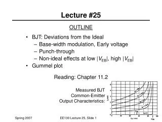
Lecture 25 Assorted Control Preparation. Block diagrams. Cruise control. Stability (the simple inverted pendulum). BLOCK DIAGRAMS. Friedland uses a lot of these. Sometimes they are helpful sometimes they are not. He gives symbols for multiply, integrate and add.

E N D
Lecture 25 Assorted Control Preparation Block diagrams Cruise control Stability (the simple inverted pendulum)
BLOCK DIAGRAMS Friedland uses a lot of these. Sometimes they are helpful sometimes they are not. He gives symbols for multiply, integrate and add We can see how this works by looking at the usual first order system block diagram
second order ode representation state space representation or simple block diagram representation - + a v y -
integrate v to get y “feedback” loops integrate the acceleration to get v - + a u y -
translated Friedland’s equations two inputs u two outputs x
The equations for that diagram are dynamics output We won’t be concerned much, if at all, with vector inputs We will not look at systems for which the output depends directly on the input — for us D = 0
Inverted pendulum on a cart which problem we will work much later m q l u M y
Energies Constraints The Lagrangian Euler-Lagrange equations
Linearize Solve for the second derivatives Convert to state space
y output B input q output internal “feedback”
CRUISE CONTROL desired speed INVERSE PLANT GOAL: SPEED nominal fuel flow Actual speed + + PLANT: DRIVE TRAIN Input: fuel flow - - error disturbance Feedback: fuel flow CONTROL
disturbance simple first order model divide the force open loop part linearize and the goal is to make v’ go to zero
Let’s say a little about possible disturbances hills are probably the easiest to deal with analytically mgsinf f I’ll say more as we go on
The open loop picture + + f v 1/m -
I’m not in a position to simply ask f to cancel h(t) (because I don’t know what it is!) I want some feedback mechanism to give me more fuel when I am going too slow and less fuel when I am going too fast This system is already stable in the sense that the air drag acts in the same way as the artificial gain I don’t really need the primes anymore, so I will drop them
The closed loop picture The open loop picture + + - f v 1/m -
From the last lecture So we have Solution
We do not need this whole apparatus to get a sense of how this works Consider a hill, for which s(t) is constant, call it s0 We can find the particular solution by inspection The homogeneous solution decays, and we see that we have a permanent error in the speed The bigger K, the smaller the error, but we can’t make it go away (and K will be limited by physical considerations in any case)
What we’ve done so far is called proportional (P) control We can fix this problem by adding integral (I) control. There is also derivative (D) control PID control incorporates all three types, and you’ll hear the term
Add a variable and its ode Let the force depend on both variables Then
Convert to state space We remember that x denotes the error so the initial condition for this problem is y = 0 = v
The homogeneous solution and we see that it will decay
What happens now when we go up a hill? We can now let the displacement take care of the particular solution
Let’s look at the behavior of first and second order cruise controls in Mathematica
Inverted pendulum on a cart which problem we will work much later for now, fix the cart: y = 0 = u m q Add a torque l M
Energies Constraints The Lagrangian Euler-Lagrange equation
Linearize Convert to state space
Look at the homogeneous solution The system is unstable If there is no torque, the pendulum will fall down
Suppose the torque depends on the angle We are introducing feedback now where it is essential
I have converted the open loop problem to a closed loop problem and said problem is a new homogeneous problem and we want the solution to decay to zero to hold the pendulum up
If the eigenvalues are pure imaginary The inverted pendulum will oscillate
In order to keep the square root part less than the outside piece so that the real part of both values of s remain negative We need both feedback elements to make hold the pendulum up
Inverted pendulum: full state feedback t - q w + -