Download
1 / 30
300 likes | 397 Vues
Creating AEW diagnostics. As seen in case studies and composites, AEWs are characterized by a ‘wavelike’ perturbation to the mid-tropospheric wind field.

E N D
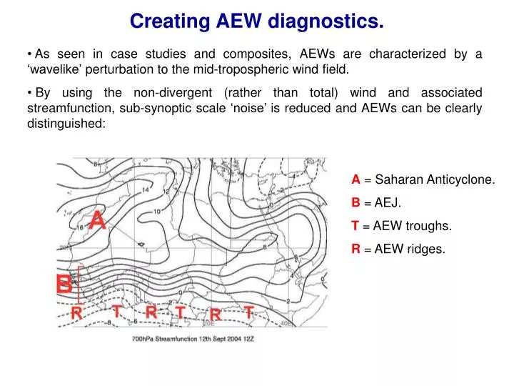
Creating AEW diagnostics. • As seen in case studies and composites, AEWs are characterized by a ‘wavelike’ perturbation to the mid-tropospheric wind field. • By using the non-divergent (rather than total) wind and associated streamfunction, sub-synoptic scale ‘noise’ is reduced and AEWs can be clearly distinguished: A = Saharan Anticyclone. B = AEJ. T = AEW troughs. R = AEW ridges.
Creating AEW diagnostics. 700hPa streamfunction and non-divergent wind (enlarged area). R T R T R • Zooming in on the AEWs and adding the non-divergent wind clearly indicates that AEW Trough and Ridges are associated with cyclonic and anticyclonic circulations.
Creating AEW diagnostics. 700hPa streamfunction and curl (vorticity) of the non-divergent wind. R T R T R • Computing the vorticity of the non-divergent wind does not depict the location of troughs/ridges clearly – primarily due to horizontal shear across the AEJ. • Simple solution: split the vorticity into its shear and curvature components.
Creating AEW diagnostics. 700hPa streamfunction with shear vorticity (black contours) and curvature vorticity (shaded) of the non-divergent wind. R T R T R • Location of the AEW troughs well depicted by shading above. • Zero contour of the shear vorticity lies at wind speed extrema: Jets and anti-jets.
Creating AEW diagnostics. 700hPa streamfunction with shear vorticity (black contours) and curvature vorticity (shaded) of the non-divergent wind. R T R T R • Synoptic reasoning: Trough or ridge lines occur when the advection of the curvature vorticity switches sign. • Jets and anti jets can be distinguished by the magnitude of the non-divergent wind and cross contour gradient of shear vorticity.
Creating AEW diagnostics. 700hPa streamfunction with advection of curvature vorticity equal zero (black solid), shear vorticity equal zero where wind speed > 8ms-1(black dashed). • Black contours clearly and accurately depict the trough/ridge and jet axes.
Creating AEW diagnostics. 700hPa streamfunction with advection of curvature vorticity equal zero (black solid), shear vorticity equal zero plus plotting masks. • Plotting masks (user variable) are added to isolate trough lines and wind speed maxima in easterly flow : the end result gives distinct AEW trough and AEJ axes.
Creating AEW diagnostics: Example. ▲315K PV (coloured) on METEOSAT IR with objective 700hPa AEW trough lines (black solid) and Easterly jet axes (black dashed), all from the GFS analysis for 12th Sept 2004.
Application of diagnostics (1). - African Easterly Wave activity. • Using rule driven methodology with manual tracking, we have generated seasonal overviews of AEW activity over the African continent for July, August, September 2004-2006. • Found that ‘mean’ AEW in both seasons had properties similar to composite structures found in literature. However, observed large amount of variability in the individual cases e.g. synoptic structure, propagation speeds (varying between 5 and 15ms-1), initiation points (varying between 35°E and 10°W). • Early results suggest that the majority (>50%) of AEWs either become tropical cyclones or are removed from the Atlantic basin by a semi-permanent trough in the central Atlantic basin. • More details in Berry, Thorncroft and Hewson (2007, MWR).
Application of diagnostics (2). -Tracking of precursor disturbances. • Application of idealized or composite AEW structure and/or nephanalysis to real AEW structures is not always straightforward. • AEWs may be highly tilted, interacting with extratropical features or may lack active deep convection, but remain potent precursor disturbances. • Combination of the diagnostics with mid-tropospheric potential vorticity (PV) can help to simplify the interpretation plus aid the identification and tracking of precursor disturbances, especially those that are weak. • Example:
315K Potential Vorticity (shaded, units tenths PVU), 700hPa streamlines, EW trough axes (solid black) and EJ axes (dashed black). Data from 0.5°x0.5°GFS analysis. W8 W9 W10 7th August 2005 00UTC
315K Potential Vorticity (shaded, units tenths PVU), 700hPa streamlines, EW trough axes (solid black) and EJ axes (dashed black). Data from 0.5°x0.5°GFS analysis. ‘Irene’ X W8 W9 W10 8th August 2005 00UTC
315K Potential Vorticity (shaded, units tenths PVU), 700hPa streamlines, EW trough axes (solid black) and EJ axes (dashed black). Data from 0.5°x0.5°GFS analysis. ‘Irene’ X W8 W9 W10 9th August 2005 00UTC
315K Potential Vorticity (shaded, units tenths PVU), 700hPa streamlines, EW trough axes (solid black) and EJ axes (dashed black). Data from 0.5°x0.5°GFS analysis. ‘Irene’ X W8 W9 W11 W10 10th August 2005 00UTC
315K Potential Vorticity (shaded, units tenths PVU), 700hPa streamlines, EW trough axes (solid black) and EJ axes (dashed black). Data from 0.5°x0.5°GFS analysis. ‘Irene’ X W8 W11 W10 11th August 2005 00UTC
315K Potential Vorticity (shaded, units tenths PVU), 700hPa streamlines, EW trough axes (solid black) and EJ axes (dashed black). Data from 0.5°x0.5°GFS analysis. ‘Irene’ X W8 W11 W10 12th August 2005 00UTC
315K Potential Vorticity (shaded, units tenths PVU), 700hPa streamlines, EW trough axes (solid black) and EJ axes (dashed black). Data from 0.5°x0.5°GFS analysis. ‘Irene’ X W11 W10 13th August 2005 00UTC
315K Potential Vorticity (shaded, units tenths PVU), 700hPa streamlines, EW trough axes (solid black) and EJ axes (dashed black). Data from 0.5°x0.5°GFS analysis. ‘TD10’ X W11 W10 14th August 2005 00UTC
315K Potential Vorticity (shaded, units tenths PVU), 700hPa streamlines, EW trough axes (solid black) and EJ axes (dashed black). Data from 0.5°x0.5°GFS analysis. W10 W11 W12 15th August 2005 00UTC
315K Potential Vorticity (shaded, units tenths PVU), 700hPa streamlines, EW trough axes (solid black) and EJ axes (dashed black). Data from 0.5°x0.5°GFS analysis. W10 W11 W12 16th August 2005 00UTC
315K Potential Vorticity (shaded, units tenths PVU), 700hPa streamlines, EW trough axes (solid black) and EJ axes (dashed black). Data from 0.5°x0.5°GFS analysis. W10 W12 W11 17th August 2005 00UTC
315K Potential Vorticity (shaded, units tenths PVU), 700hPa streamlines, EW trough axes (solid black) and EJ axes (dashed black). Data from 0.5°x0.5°GFS analysis. (W10) W13 W11 18th August 2005 00UTC
315K Potential Vorticity (shaded, units tenths PVU), 700hPa streamlines, EW trough axes (solid black) and EJ axes (dashed black). Data from 0.5°x0.5°GFS analysis. (W10) W13 19th August 2005 00UTC
315K Potential Vorticity (shaded, units tenths PVU), 700hPa streamlines, EW trough axes (solid black) and EJ axes (dashed black). Data from 0.5°x0.5°GFS analysis. W10 W13 20th August 2005 00UTC
315K Potential Vorticity (shaded, units tenths PVU), 700hPa streamlines, EW trough axes (solid black) and EJ axes (dashed black). Data from 0.5°x0.5°GFS analysis. (W10) W13 21st August 2005 00UTC
315K Potential Vorticity (shaded, units tenths PVU), 700hPa streamlines, EW trough axes (solid black) and EJ axes (dashed black). Data from 0.5°x0.5°GFS analysis. W10 W13 22nd August 2005 00UTC
315K Potential Vorticity (shaded, units tenths PVU), 700hPa streamlines, EW trough axes (solid black) and EJ axes (dashed black). Data from 0.5°x0.5°GFS analysis. W10 W13 23rd August 2005 00UTC
315K Potential Vorticity (shaded, units tenths PVU), 700hPa streamlines, EW trough axes (solid black) and EJ axes (dashed black). Data from 0.5°x0.5°GFS analysis. X ‘Katrina’ W10 W13 24th August 2005 00UTC
315K Potential Vorticity (shaded, units tenths PVU), 700hPa streamlines, EW trough axes (solid black) and EJ axes (dashed black). Data from 0.5°x0.5°GFS analysis. X ‘Katrina’ W10 W13 25th August 2005 00UTC
Application of diagnostics (3). - NWP comparison and verification. • Succinct representation of synoptic features given by our diagnostics allows easy comparison of the performance of different model analyses or forecasts. • “Spaghetti” diagrams of diagnostics helps gauge the confidence associated with the forecast or analysis of a particular synoptic feature. 700hPa EW Troughs axes GFS 700hPa Easterly Jet axes GFS