Download
1 / 105
1.18k likes | 1.7k Vues
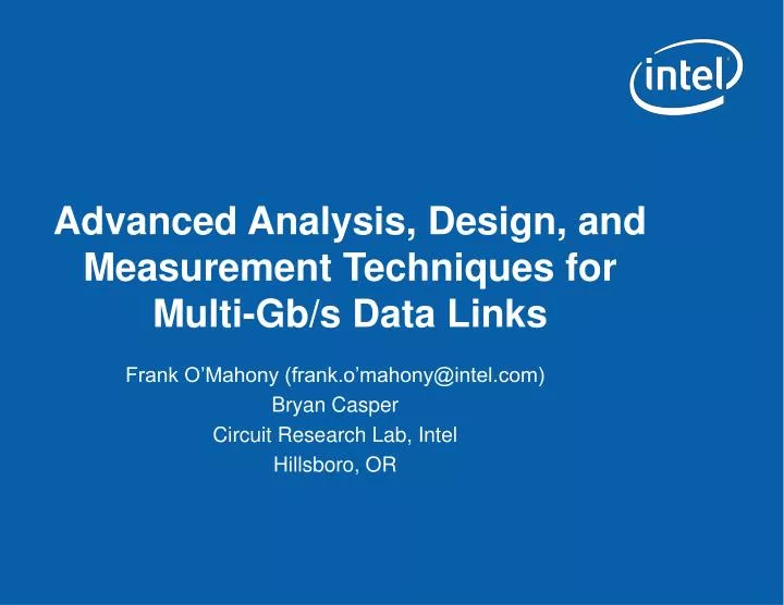
Advanced Analysis, Design, and Measurement Techniques for Multi-Gb/s Data Links . Frank O’Mahony (frank.o’mahony@intel.com) Bryan Casper Circuit Research Lab, Intel Hillsboro, OR. Outline. Overview of I/O trends System-level link modeling Worst-case data eye Statistical data eye

E N D
Advanced Analysis, Design, and Measurement Techniques for Multi-Gb/s Data Links Frank O’Mahony (frank.o’mahony@intel.com) Bryan Casper Circuit Research Lab, Intel Hillsboro, OR
Outline • Overview of I/O trends • System-level link modeling • Worst-case data eye • Statistical data eye • Design example: 20Gb/s link • On-die measurement techniques
… noise Channel Sampler Slicer Linear Equalizer Transmit Filter h(t) S CDR Chip-to-Chip Signaling Trends Decade Speeds Transceiver Features 1980’s >10Mb/s Inverter out, inverter in 1990’s >100Mb/s Termination Source-synchronous clk. 2000’s >1 Gb/s Pt-to-pt serial streams Pre-emphasis equalization Future >10 Gb/s Adaptive Equalization, Advanced low power clk. Alternate channel materials Lumped capacitance Transmission line Lossy transmission line
CMOS transceiver data rates • Plot showing link rate vs. year Power/channel limitations Technology limited Courtesy of Prof. Ken Yang, UCLA
Sun's Surface Rocket Nozzle Nuclear reactor Hot plate Power Density Increases Exponentially! 1000 Max power density envelope 100 Pentium® 4 Power density [Watts/cm2] Pentium® III Pentium® II 10 Pentium® Pro Pentium® i386 i486 1 1.5 1 0.7 0.5 0.35 0.25 0.18 0.13 0.1 0.07 Process Technology node [μm]
Teraflops Research Chip100 Million Transistors ● 80 Tiles ● 275mm2 • First tera-scale programmable silicon: • Teraflops performance • Tile design approach • On-die mesh network • Power-aware capability • Tera-scale many-core μP’s will drive aggregate I/O rates aggressively
Power efficiency and process technology • Process scaling enables lower power data links • Channel characteristics can limit achievable power efficiency Courtesy of Prof. Ken Yang, UCLA
I/O Data Rate and Power Efficiency 60 40 Power Efficiency (mW/Gb/s) 20 11.7 9.6 7.5 Prete ISSCC’07 J. Wong VLSI’03 R. Palmer ISSCC’07 BNV ISSCC’06 2.2 0 0 5 10 15 20 Data Rate (Gb/s)
Designing power-efficient multi-Gb/s links • Accurate system-level link modeling • Careful statistical accounting of all noises • ISI, Xtalk, voltage, and timing noise • Power-efficient I/O system implementation • Design within the BW of the process technology • Better channel characteristics enable lower power • Immunity to variation, deterministic and random noise comes at a power cost • On-die calibration and measurement • Calibration can significantly reduce power • Measurement necessary to close the modeling loop
System-level link modeling • Empirical calculation • Use random data • Peak distortion analysis • Analytical calculation of worst-case eye • Statistical ISI analysis • Analytical calculation of BER eye
Traditional method of signaling analysis and validation • Most chip-to-chip signaling links considered in the past used simple Binary NRZ modulation • These links had a low symbol rate and little channel memory • Transient simulation using a few random data vectors was sufficient to accurately characterize the eye.
Motivation for behavioral link analysis • Simulated eye can be optimistic • Won’t capture worst-case ISI, especially for channels with long memory • Characterizes impact of deterministic and random noise sources • For low bit error rates (BER), very unlikely noise conditions must be considered • Nearly exact statistical analysis reduces need for excess design margins • Fast evaluation of various link architectures without designing complete circuits • e.g. Various equalizers can be traded off easily
FFT Impulse Response Convolution Superposition Frequency response (e.g. S-parameters) S21 Impulse Response Properties of a Linear Time-invariant System
LTI property: Convolution Tx symbol (mirror) Impulse response Pulse response
LTI property: Superposition Out In Tx symbol …000010000000… Pulse response
Response to pattern 100111 LTI property: Superposition of symbols Out In Tx symbol … 000010011100 …
FEXT Pulse response LTI property: Superposition of coupled symbols In Out Tx symbol …000010000000…
FEXT response LTI property: Superposition of coupled symbols In Out Tx symbol …000011111100…
FEXT response LTI property: Superposition of coupled symbols Out Tx symbol …000011111100…
Insertion loss response LTI property: Superposition of coupled symbols Out Tx symbol …000010011100…
FEXT response Insertion loss response Composite response LTI property: Superposition of coupled symbols Out Tx symbol …000011111100… Tx symbol …000010011100…
Worst-case eye calculation • Eye diagrams are generally calculated empirically • Convolve random data with pulse response of channel • Pulse response is derived by convolving the impulse reponse with the transmitted symbol • For eye diagrams to represent the worst-case, a large set of random data must be used • Low probability of hitting worst case data transitions • Computationally inefficient • An analytical method of producing the worst-case eye diagram exists • Computationally efficient algorithm
Eye diagram (1000 bits @5Gb/s) Random data eye (100 bits) --- Random data eye (1000 bits) ---
ISI+ ISI- precursor cursor postcursor Sample pulse response
0 0 0 0 1 1 1 1 1 1 1 1 1 1 1 Step response
0 1 1 0 1 0 0 1 0 0 0 0 0 Worst-case 0
0 1 0 1 1 0 0 0 0 0 Worst-case 1
How to find worst-case patterns Worst-case 0 1 1 0 1 0 0 1 Worst-case 1 0 0 1 0 1 1 0
2 16 -3 4 -1 2 2 Worst-case Received Voltage Difference (RVD)
Worst-case 1 Worst-case 0 5Gb/s Response due to worst-case data pattern
Lone 1 Worst-case 1 Worst-case data response
5Gb/s WC eye shape PrecursorCursorPostcursor
WC eye vs random data eye WC eye shape 100 symbols random data eye 1000 symbols random data eye
Sample time BER distribution eye Legend Sample reference Sample voltage (V) BER in 10X Sample time (sec) What is a BER distribution eye? BER=10-10
Sample time BER distribution eye Legend Sample reference Sample voltage (V) BER in 10X Sample time (sec) What is a BER distribution eye? BER=10-5
Sample time BER distribution eye Legend Sample reference Sample voltage (V) BER in 10X Sample time (sec) What is a BER distribution eye? BER=10-1
BER distribution vs Worst-case eye Worst-case eye edges Legend shows BER in 10X
BER distribution eye calculation • Calculation method is based on pulse response shape • Assumption: Equal probability of 1 or 0 • Determine probability density function (pdf) of ISI • In contrast to determining peak value of ISI • More computationally intensive than Peak Distortion Analysis
BER eye calculation example (no ISI) 0 0 9 0 0 0 0
9 1 0 1 PDF of cursor for a 1 PDF of ISI PDF of the cursor (when sending a 1)
Convolve PDFs PDF of cursor for a 1 PDF of ISI PDF of a 1 9 0 9 PDF of a 1
Cumulative Distribution Function (CDF) of a 1 PDF of a 1 9 9
BER distribution eye (when sampling a 1) Legend (BER): 1 0 9 CDF of a 1 0 9
Convolve PDFs PDF of ISI PDF of cursor for a 0 PDF of a 0 0 0 0 PDF of a 0
Cumulative Distribution Function (CDF) of a 0 PDF of a 0 0 0
BER distribution eye (when sampling a 0) Legend (BER): 1 0 9 CDF of a 0 0 0