Download

1 / 29
290 likes | 436 Vues
Daniel Jansson. Stopband constraint case and the ambiguity function. Stopband constraint case. Goal Generate discrete, unimodular sequences with frequency notches and good correlation properties Why?

E N D
Daniel Jansson Stopband constraint case and the ambiguity function
Stopband constraint case Goal Generate discrete, unimodular sequences with frequency notches and good correlation properties Why? Avoiding reserved frequency bands is important in many applications (communications, navigation..) Avoiding other interference How? SCAN (Stopband CAN) / WeSCAN (Weighted Stopband CAN)
Stopband CAN (SCAN) Let {x(n)}, n = 1...N be the sought sequence Express the bands to be avoided as Define the DFT matrix with elements Form matrix S from the columns of FÑcorresponding to the frequencies in Ω We suppress the spectral power of {x(n)} in Ω by minimizingwhere
Stopband CAN (SCAN) The problem on the previous slide is equivalent towhere G are the remaining columns of FÑ. Suppressing the correlation sidelobes is done using the CAN formulation
Stopband CAN (SCAN) Combining the frequency band suppression and the correlation sidelobe suppression problems we getwhere 0 ≤ λ ≤ 1 controls the relative weight on the two penalty functions. The problem is solved by using the algorithm on the next slide
Stopband CAN (SCAN) If a constrained PAR is preferable to unimodularity the problem can be solved in the same way except x for each iteration is given by the solution to
Weighted SCAN (WeSCAN) Minimization of J2 is a way of minimizing the ISL The more general WISL (weighted ISL) is given bywhere are weights
Weighted SCAN (WeSCAN) Let and D be the square root of Γ. Then the WISL can be minimized by solvingwhereand Replace in the SCAN problem with and perform the SCAN algorithm, but do necessary changes that are straightforward.
Numerical examples The spectral power of a SCAN sequence generated with parameters N = 100, Ñ = 1000, λ = 0.7 andΩ = [0.2,0.3] Hz. Pstop = -8.3 dB (peak stopband power)
Numerical examples The autocorrelation of a SCAN sequence generated with parameters N = 100, Ñ = 1000, λ = 0.7 andΩ = [0.2,0.3] Hz, Pcorr = -19.2 dB (peak sidelobe level)
Numerical examples Pstop and Pcorrvsλ
Numerical examples The spectral power of a WeSCAN sequence generated with γ1=0, γ2=0 and γk=1 for larger k. Pstop = -34.9 dB (peak stopband power)
Numerical examples The autocorrelation of the WeSCAN sequence
Numerical examples The spectral power of a SCAN sequence generated with PAR ≤ 2
The Ambiguity Function The response of a matched filter to a signal with various time delays and Doppler frequency shifts (extension of the correlation concept). The (narrowband) ambiguity function iswhere u(t) is a probing signal which is assumed to be zero outside [0,T], τis the time delay and f is the Doppler frequency shift.
The Ambiguity Function Three properties worth noting The maximum value of |χ(τ,f)| is achieved at | χ(0,0)| and is the energy of the signal, E d|χ(τ,f)|= |χ(-τ,-f)| D
The Ambiguity Function Proofs Cauchy-Schwartz givesand since | χ(0,0)| = E, property 1 follows. Use the variable change t -> t+ τwhich implies property 2.
The Ambiguity Function Proofs 3. The volume of |χ(τ,f)|2is given byLet Wτ(f) be the Fourier transform of u(t)u*(t- τ). Parseval givestherefore
The Ambiguity Function Ambiguity function of a chirp
The Ambiguity Function Ambiguity function of a Golomb sequence
The Ambiguity Function Ambiguity function of CAN generated sequences
The Ambiguity Function Why is there a vertical stripe at the zero delay cut? The ZDC is nothing but the Fourier transform of u(t)u*(t). Since u(t) is unimodular we getand the sinc-function decreases quickly as f increases. No universal method that can synthesize an arbirtrary ambiguity function.
The Discrete AF Assume u(t) is on the formwhere pn(t) is an ideal rectangular pulse of lengthtp The ambiguity function can be written as Inserting τ = ktpand f = p/(Ntp) giveswhere is called the discrete AF. If |p|<<N then
The Discrete AF Minimizing the sidelobes of the discrete AF in a certain regionwhere and are the index sets specifying the region. Define the set of sequences as
The Discrete AF Denote the correlation between {xm(n)} and {xl(n)} by All values of are contained in the set Minimizing the correlations is thus equivalent to minimizing the discrete AF sidelobes.
The Discrete AF Define where All elements of appear in We can thus minimizewhich as we saw before is almost equivalent to Minimize by using the cyclic algorithm on the next slide