Download
1 / 11
110 likes | 298 Vues
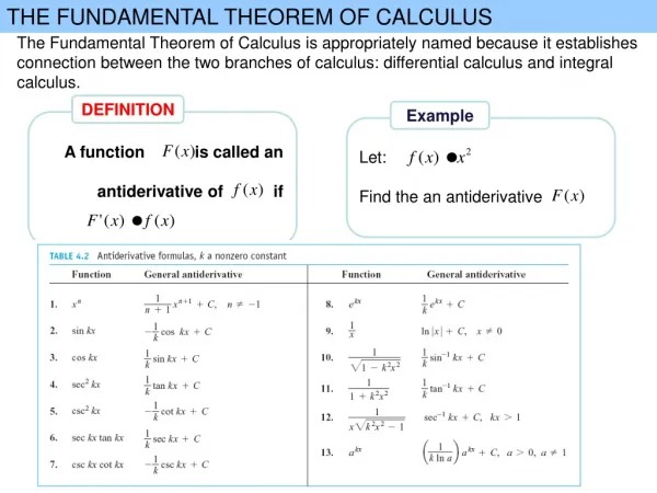
The Fundamental Theorem of Calculus . This power point presentation is created and written by Dr. Julia Arnold Using the 5 th edition of S. T. Tan’s text Applied Calculus. History:. Georg Friedrich Bernhard Riemann

E N D
The Fundamental Theorem of Calculus This power point presentation is created and written by Dr. Julia Arnold Using the 5th edition of S. T. Tan’s text Applied Calculus
History: Georg Friedrich Bernhard Riemann Born: 17 Sept 1826 in Breselenz, Hanover (now Germany)Died: 20 July 1866 in Selasca, Italy The summation of the rectangles under a curve was called a Riemann sum in honor of this German mathematician. For more information goto: http://www-groups.dcs.st-and.ac.uk/~history/Mathematicians/Riemann.html
More History: Gottfried Wilhelm Leibniz Gottfried Wilhelm Leibniz (b. 1646, d. 1716) was a German philosopher, mathematician, and logician who is probably most well known for having invented the differential and integral calculus (independently of Sir Isaac Newton). In his correspondence with the leading intellectual and political figures of his era, he discussed mathematics, logic, science, history, law, and theology. For more information goto: http://mally.stanford.edu/leibniz.html
More History Sir Isaac Newton Isaac Newton is perhaps the best known renaissance scientist today, living between 1642 and 1727. We think of gravity, celestial mechanics, and calculus when we think of him. He certainly did develop the calculus by building upon the ideas of Fermat and Barrow (the person whose chair he took when he went to Cambridge). But he was not alone in developing calculus (see next). And his focus was really one of mechanics - how do bodies move. His focus was always on motion and is reflected in the terminology he chose for calculus - what we call "derivatives", he called "fluxions". And his integrals were simply "inverse fluxions". You can see how "flux" was his focus. He also developed the "dot" notation for calculus - one dot meant a first derivative, two dots a second, and so forth. Today this is used, but only with respect to time derivatives. A general derivative still needs to specify the variable of differentiation and more often than not, time derivatives are done in this more general manner.As indicated earlier, For more goto: http://www.chembio.uoguelph.ca/educmat/CHM386/RUDIMENT/tourclas/newton.htm
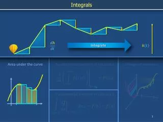
Example 1: Let f(x)= 3x and let us fine the area under the curve and between the vertical lines x = 1 and x = 3 and bounded also by the x-axis. Since the area we need to find is a trapezoid, we could first find the area geometrically, and then use the FTofC. I bet you don’t remember what the formula is for the area of a trapezoid. A= ½ (b1 + b2)h
Example 1: Let f(x)= 3x and let us fine the area under the curve and between the vertical lines x = 1 and x = 3 and bounded also by the x-axis. A= ½ (b1 + b2)h The bases b1 and b2 are the parallel sides and h is the perpendicular distance between them. b2 b1 = 3 and b2 =9 h = 2 A= ½ (3 + 9)2=12 b1 h
Example 1: Let f(x)= 3x and let us fine the area under the curve and between the vertical lines x = 1 and x = 3 and bounded also by the x-axis. Now let’s use the FTofC
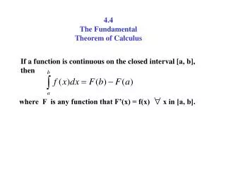
Since Example 1 verifies the accuracy of this method, let’s go for something more intriguing. Remember this problem from 6.3 We found that the area under the curve was between 3 and 7. Not very close. To do better we need to construct more partitions. Let’s integrate
Since Example 1 verifies the accuracy of this method, let’s go for something more intriguing. Remember this problem from 6.3 We found that the area under the curve was between 3 and 7. Not very close. To do better we need to construct more partitions. Let’s integrate
Example 3. Find the area under the curve y = x2 + 1 from x = -1 to x = 2. Solution: Note: You must make sure that the area is above the x-axis and none is below.
Evaluate the definite integral Solution: Because of our limitation of rules, we should multiply the two factors before integrating.