Download
1 / 44
440 likes | 620 Vues
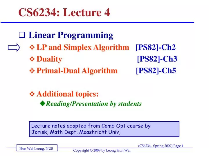
CS6234: Lecture 4. Linear Programming LP and Simplex Algorithm [PS82]-Ch2 Duality [PS82]-Ch3 Primal-Dual Algorithm [PS82]-Ch5 Additional topics: Reading/Presentation by students. Lecture notes adapted from Comb Opt course by Jorisk, Math Dept, Maashricht Univ,.

E N D
CS6234: Lecture 4 • Linear Programming • LP and Simplex Algorithm [PS82]-Ch2 • Duality [PS82]-Ch3 • Primal-Dual Algorithm [PS82]-Ch5 • Additional topics: • Reading/Presentation by students Lecture notes adapted from Comb Opt course by Jorisk, Math Dept, Maashricht Univ,
Comments by LeongHW: First review some old transparencies…
Chapter 2 The Simplex Algorithm (Linear programming) Combinatorial Optimization Masters OR
General LP Given: m x n integer Matrix, A, with rows a’i. M set of rows corresponding to equality constraints M’set of rows corresponding to inequality constraints x ε Rn N set of columns corresponding to constraint variables, N’ set of colums corresponding to unconstraint variables. m-vector b of integers, n-vector c of integers Combinatorial Optimization Masters OR
General LP (cont.) Definition 2.1 An instance of general LP is defined by min c’ x s.t. a’i = bi i ε M a’i ≤ bi i ε M’ xj ≥ 0 j ε N xjfree j ε N’ Combinatorial Optimization Masters OR
Other forms of LP Canonical form min c’ x s.t. Ax ≥ r x ≥ 0 Standard form min c’ x s.t. Ax = b x ≥ 0 It is possible to reformulate general forms to canonical form and standard form and vice versa. The forms are equivalent (see [PS]) Combinatorial Optimization Masters OR
Linear algebra basics Definition 0.1Two or more vectors v1, v2, ...,vmwhich are not linearly dependent, i.e., cannot be expressed in the form d1v1 + d2v2 +...+ dmvm = 0 with d1, d2 ,..., dm, constants which are not all zero are said to be linearly independent. Definition 0.2A set of vectors v1, v2, ...,vm is linearly independent iff the matrix rank of the matrix V = (v1, v2, ...,vm) is m, in which case V is diagonazible. Combinatorial Optimization Masters OR
Linear Algebra basics (cont.) Definition 0.3A square m x m matrix of rank m is called regular or nonsingular. A square m x m matrix of rank less than m is called singular. Alternative definition A square m x m matrix is called singular if its determinant equals zero. Otherwise it is called nonsingular or regular. Combinatorial Optimization Masters OR
Basis Assumption 2.1 Matrix A is of Rank m. Definition 2.3A basis of A is a linearly independent collection Q = {Aj1,...,Ajm}. Thus Q can be viewed as a nonsingular Matrix B. The basic solution corresponding to Q is a vector x ε Rn such that = k-th component of B-1b for k =1,…,m, xjk = 0 otherwise. Combinatorial Optimization Masters OR
Finding a basic solutionx • Choose a set Q of linearly independent columns of A. • Set all components of x corresponding to columns not in Q to zero. • Solve the m resulting equations to determine the components of x. These are the basic variables. Combinatorial Optimization Masters OR
Basic Feasible Solutions Definition 2.4: If a basic solution is in F, then is a basic feasible soln (bfs). Lemma 2.2: Let x be a bfs of Ax = b x ≥ 0 corresponding to basis Q. Then there exists a cost vector c such that x is the unique optimal solution of min c’ x s.t. Ax = b x ≥ 0 Combinatorial Optimization Masters OR
Lemma 2.2 (cont.) Proof: Choose cj = 0 if Ajε B, 1 otherwise. Clearly c’ x = 0, and must be optimal since all coefficients of c are non-negative integers. Now consider any other feasible optimal solution y. It must have yj=0 for all Ajnot in B. Therefore y must be equal to x. Hence x is unique. Combinatorial Optimization Masters OR
Existence of a solution Assumption 2.2: The set F of feasible points is not empty. Theorem 2.1: Under assumptions 2.1. and 2.2 at least one bfs exists. Proof. [PS82] Combinatorial Optimization Masters OR
And finally on feasible basic solutions Assumption 2.3 The set of real numbers {c’x : x ε F} is bounded from below. Then, using Lemma 2.1, Theorem 2.2 (which you may both skip) derives that x can be bounded from above, and that there is some optimal value of its cost function. Combinatorial Optimization Masters OR
Geometry of linear programming Definition 0.4. A subspaceS of Rd is the set of points in Rd satisfying a set of homogenous equations S={x ε Rd: aj1 x1 + aj2 x2 + .....+ ajd xd =0, j=1...m} Definition 0.5.The dimension dim(S) of a subspace S equals the maximum number of independent vectors in it. Dim(S) = d-rank(A). Combinatorial Optimization Masters OR
Geometry of linear programming Definition 0.6. An affine subspaceS of Rd is the set of points in Rd satisfying a set of nonhomogenous equations S = {x ε Rd: aj1 x1 + aj2 x2 + .....+ ajd xd =bj, j=1...m} Consequence: The dimension of the set F defined by the LP min c’ x s.t. Ax = b, A an m x d Matrix x ≥ 0 is at most d-m Combinatorial Optimization Masters OR
Convex Polytopes Affine subspaces: a1x1 + a2x2 =b a1x1 + a2x2 + a3x3 = b x2 x1 x3 x2 x1 Combinatorial Optimization Masters OR
Convex polytopes Definition 0.7 An affine subspace a1x1 + a2x2 + + adxd = b of dimension d-1 is called a hyperplane. A hyperplane defines two half spaces a1x1 + a2x2 + + adxd ≤ b a1x1 + a2x2 + + adxd ≥ b Combinatorial Optimization Masters OR
Convex polytopes A half space is a convex set. Lemma 1.1 yields that the intersection of half spaces is a convex set. Definition 0.8 If the intersection of a finite number of half spaces is bounded and non empty, it is called a convex polytope, or simply polytope. Combinatorial Optimization Masters OR
Example polytope Theorem 2.3 Every convex polytope is the convex hull of its vertices Convention: Only in non-negative orthant d equations of the form xj ≥ 0. Combinatorial Optimization Masters OR
Convex Polytopes and LP A convex polytope can be seen as: • The convex hull of a finite set of points • The intersection of many halfspaces • A representation of an algebraic system Ax = b, where A an m x n matrix x ≥ 0 Combinatorial Optimization Masters OR
Cont. Since rank(A) = m, Ax = b can be rewritten as xi = bi – Σj=1n-m aij xj i=n-m+1,...,n Thus, F can be defined by bi – Σj=1n-m aij xj ≥ 0 i=n-m+1,...,n xj ≥ 0 j=1,..,n-m The intersection of these half spaces is bounded, and therefore this system defines a convex polytope P which is a subset of Rn-m. Thus the set F of an LP in standard form can be viewed as the intersection of a set of half spaces and as a convex polytope. Combinatorial Optimization Masters OR
Cont. Conversely let P be a polytope in Rn-m. Then n half spaces defining P can be expressed as hi,1x1 + hi,2x2 + … + hi,n-mxn-m + gi ≤ 0, i =1..n. By convention, we assume that the first n-m inequalities are of the form xi ≥ 0. Introduce m slack variables for the remaining inequalities to obtain Ax = b where A an m x n matrix x ≥ 0 Where A = [H | I] and x ε Rn. Combinatorial Optimization Masters OR
Cont. Thus every polytope can indeed be seen as the feasible region of an LP. Any point x* = (x1 x2,,.., xn-m) in P can be transformed to x = (x1 x2,,.., xn) by letting xi = – gi –Σj-1n-m hij xj, i = n+m-1,...,n. (*) Conversely any x = (x1 x2,,.., xn) ε F can be transformed to x* = (x1 x2,,.., xn-m) by truncation. Combinatorial Optimization Masters OR
Vertex theorem Theorem 2.4: Let P be a convex polytope, F = {x : Ax=b, x≥0} the corresponding feasible set of an LP and x* = (x1 x2,,.., xn-m)ε P. Then the following are equivalent: • The point x*is a vertex of P. • x*cannot be a strict convex combination of points of P. • The corresponding vector x as defined in (*) is a basic feasible solution of F. Proof: DIY, [Show abca] (see [PS82]) Combinatorial Optimization Masters OR
A glimpse at degeneracy Different bfs’s lead to different vertices of P (see proof from c a), and hence lead to to different bases, because they have different non-zero components. However in the augmentation process from ab different bases may lead to the same bfs. Combinatorial Optimization Masters OR
x1 + x2 + x3 ≤ 4 x1 ≤ 2 x3 ≤ 3 3x2 + x3 ≤ 6 x1 ≥ 0 x2 ≥ 0 x3 ≥ 0 Example Combinatorial Optimization Masters OR
x1 + x2 + x3 +x4 = 4 x1 +x5 = 2 x3 +x6 = 3 3x2 + x3 +x7 = 6 First basis: A1,A2,A3,A6. x1=2,x2=2,x6=3. Example (cont.) Second basis: A1,A2,A4,A6. x1=2,x2=2,x6=3 Combinatorial Optimization Masters OR
Example (cont.) x1 + x2 + x3 ≤ 4 x1 ≤ 2 x3 ≤ 3 3x2 + x3 ≤ 6 x1 ≥ 0 x2 ≥ 0 x3 ≥ 0 Combinatorial Optimization Masters OR
Degeneracy Definition 2.5 A basic feasible solution is called degenerate if it contains more than n-m zeros. Theorem 2.5 If two distinct bases correspond to the same bfs x, then x is degenerate. Proof: Suppose Q and Q’ determine the same bfs x. Then they must have zeros in the columns not in Q, but also in the columns Q\Q’. Since Q\Q’ is not empty, x is degenerate. Combinatorial Optimization Masters OR
Optimal solutions Theorem 2.6: There is an optimal bfs in any instance of LP. Furthermore, if q bfs’ are optimal, so are the convex combinations of these q bfs’s. Proof: By Theorem 2.4 we may alternatively proof that the corresponding polytope P has an optimal vertex, and that if q vertices are optimal, then so are their convex combinations. Assume linear cost = d’x. P is closed and bounded and therefore d attains its minimum in P. Combinatorial Optimization Masters OR
Cont. Let xo be a solution in which this minimum is attained and let x1,...,xn be the vertices of P. Then, by Theorem 2.3, xo = ΣNi=1αi xiwhereΣNi=1αi = 1, αi ≥ 0. Let xj be the vertex with lowest cost. Then d’xo = ΣNi=1αi d’xi ≥ d’xiΣNi=1αi = d’xi, and therefore xj is optimal. This proofs the first part of the Theorem. For the second part,notice that if y is a convex combination of optimal vertices x1,x2,..xq, then, since the objective function is linear, y has the same objective function value and is also optimal. Combinatorial Optimization Masters OR
Moving from bfs to bfs Let x0 = {x10,…,xm0} be such that Σi xi0 Ab(i) = b (1) Let B be the corresponding basis, (namely, set of columns {AB(i) : i =1,…m} Then every non basic column Aj can be written as Σi xij AB(i) = Aj (2) Together this yields: Σi (xi0 – θ xij )AB(i) + θ Aj = b. Combinatorial Optimization Masters OR
Moving from bfs to bfs (2) Consider Σi(xi0 – θ xij)AB(i) + θ Aj = b Now start increasing θ. This corresponds to a basic solution in which m+1 variables are positive (assuming x is non-degenerate). Increase θ until at least one of the (xi0 – θ xij) becomes zero. We have arrived at a solution with at mostm non-zeros. Another bfs Combinatorial Optimization Masters OR
Simplex Algorithm in Tableau 3x1 + 2x2 + x3 = 1 5x1 + 2x2 + x3 + x4 = 3 2 x1 + 5 x2 + x3 + x5 = 4 Combinatorial Optimization Masters OR
Tableau Basis diagonalized Moving to other bfs Bfs {x3=1, x4=2, x5=3} = { xi0 }. From Tableau 2, A1 = 3A3 + 2A4 – A5 = Σ xi1AB(i) To bring column 1 into basis, θ0 = min { 1/3, 2/2 } = 1/3 corresponding to row1 (x3) leaving the basis Combinatorial Optimization Masters OR
Choosing a Profitable Column The cost of a bfs x0 = {x10,…,xm0} with basis B is given by z0 = Σi xi0 cB(i) Now consider bring a non-basic column Aj into the basis. Recall that Aj can be written as Aj = Σi xij AB(i)(2) Interpretation: For every unit of the variable xj that enters the new basis, an amount of xij of each variable xB(i) must leave. Nett change in cost (for unit increase of xj) is cj – Σi xij cB(i) Combinatorial Optimization Masters OR
Choosing a Profitable Column (2) Nett change in cost (for unit increase of xj) is c~j = cj – zj where zj = Σi xij cB(i) Call this quantity the relative cost for column j. Observations: * It is only profitable to bring in column j if c~j < 0. * If c~j 0, for all j, then we reached optimum. Combinatorial Optimization Masters OR
Optimal solutions Theorem 2.8: (Optimality Condition) At a bfs x0, a pivot step in which xj enters the basis changes the cost by the amount θ0c~j = θ0(cj – zj) If c~= (c – z) 0, then x0 is optimal. Combinatorial Optimization Masters OR
Tableau (example 2.6) Min Z = x1 + x2 + x3 + x4 + x5 s.t. 3x1 + 2x2 + x3 = 1 5x1 + 2x2 + x3 + x4 = 3 2 x1 + 5 x2 + x3 + x5 = 4 Combinatorial Optimization Masters OR
Simplex Algorithm (Tableau Form) Diagonalize to get bfs { x3, x4, x5 } Determine reduced cost by making c~j = 0 for all basic col Combinatorial Optimization Masters OR
Simplex Algorithm (Tableau Form) Bring column 2 into the basis; select pivot element and get the new basis; OPTIMAL! (since c~ > 0) Combinatorial Optimization Masters OR
Remainder of the Chapter Ch 2.7: Pivot Selection & Anti-Cycling Ch 2.8: Simplex Algorithm (2-phase alg) Combinatorial Optimization Masters OR
Thankyou. Q & A