Optimization: Introduction to Linear Programming

1. DADSS Optimization: Introduction to Linear Programming

2. Administrative Details • Exam 2 results soon(ish) • Homework 9 posted • Final project presentations two weeks • Rest of semester: • Linear programming & Optimization

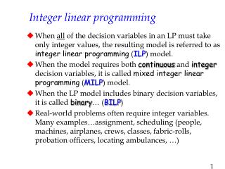
3. Optimization and Linear Programming • “Mathematical Programming” is a class of methods for solving problems that ask you to optimize: to maximize, to minimize, to find the best, the worst, the most, the least, the fastest, the shortest, etc. • Linear programming is the simplest form, suitable only for problems with linear objective functions and constraints • Two of the basic linear programming problems: • The Product Mix Problem • What quantities of products should be produced to maximize profit? • Optimal allocation of scarce resources • The Blending Problem • What combination of ingredients minimizes cost?

4. Some Optimization Basics • Unconstrained: • Unconstrained: • In general, what are we doing? • Set the derivative to zero and solve • Why? Easy: Still Easy:

5. Necessary and Sufficient Conditions

6. Some Complications • What about more complicated functions? • Calculus still works, but is cumbersome to do by hand • What about constraints? • Again, calculus works (the Lagrangian) for small problems, but requires automation for larger problems

7. More Complications Multiple Optima Discontinuous Functions f(x) f(x) x x Uncertainty Integer Restrictions f(x) f(x) x x

8. The Need for Algorithmic Methods • How can we automate searching for optima? • Linear programming (LP) is one such method • LP is fast and easy, but it has some important limitations

9. LP Structure • Assuming that the requirements for LP have been met, what does a LP look like? • Decision Variables • Quantities to be allocated • Number of units to be produced • Time intervals, unit quantities, proportions… • What does the decision maker have control over? • Objective Function • What is being maximized or minimized? • How do we reduce the world to a set of linear equations? • Constraints • (In)equalities specifying limits on the unbounded optimization of a function • If P = P × Q, why not just set Q to ∞?

10. Setting up a LP Problem: Product Mix • QElectronics makes two models of television sets, A and B. QElectronics’ profit, PA, on A is $300 per set and its profit on B, PB, is $250 per set. Thus the problem facing QElectronics is: • Notice that unconstrained optimization would cause them to produce only A! But, QElectronics faces several constraints: • Labor: They can’t use more than 40 hours of labor per day (5 full-time employees) • Manufacturing: They only have 45 hours of machine time available • Marketing: They can’t sell more than 12 units of set A per day

11. Identifying the Problem Variables • Decision Variables • What can we vary? • xA and xB are the only variables we have direct control over • Objective Function • What are we maximizing (minimizing)? • Profit! (Cost?) • A Thought: Max Profit = Min Cost = Max –Cost = … • How is it determined? • We know that PA = $300 and PB = $250, so the objective function is:

12. Identifying the Constraints 3 primary constraints plus feasibility: • Labor: A needs 2 hours of labor. B needs only 1 hour. Total labor is equal to the number of units times the labor required per unit • Manufacturing: A needs 1 hour of machine time. B needs 3 hours • Marketing: Can’t sell more than 12 units of A per day • Feasibility: Can’t make negative sets

13. The Entire LP and its Implications • What if xA or xB = 7.4235? What does it mean to produce 0.4235 TV sets? • Can 0.6689 people be employed? such that:

14. Solving LPs • Often, setting up LPs is the hardest part, because the actual “solving” is done by computer • How do computers do it? • We will use a graphical technique to illustrate the intuition behind the algorithmic methods used in optimization software packages • For any LP, there exists an infinite number of possible solutions • Problem spaces may be vast; many models have tens of thousands of variables and constraints • How can we search? How can we limit the number of possibilities we have to try?

15. Algorithmic Solutions • The Simplex Algorithm (and variants) • Created by George Dantzig in 1947 for the Air Force Office of Scientific Research • “If the LP problem has an optimal solution, it will be found in a finite number of iterations” (NB: this isn’t always very comforting) • The simplex algorithm finds the solution by making iterated improvements from an initial position • The Ellipsoid Algorithm • The best known example is Karmarkar’s Algorithm (developed at Bell Labs) • Runs in linear time • Faster than the simplex for very large problems

16. What About Solver? • Do not use Excel’s Solver as a black box! Know what’s going on underneath the surface. Remember: you will always get an answer back from Solver. However, knowing whether or not that answer is relevant requires understanding what Solver is doing. Know its limitations! • Linear programs: standard simplex • Quadratic programs: modified simplex (QP is technically NLP, but results specific to quadratic forms can be exploited to allow for significant simplification) • Nonlinear programs: Generalized Reduced Gradient method. Note: Unless you check the “assume linear model” box, Solver will automatically use GRG2. GRG2 may have difficulty with some LP or QP problems that could have more easily been solved by another method • Integer programs: Branch and Bound

17. Solution Method Intuition • All of the solution methods just mentioned tend to have very intuitive explanations • We will talk about how the simplex method works by graphically solving a small (two variable) linear program • The problem: such that:

18. Graphical Solutions • Limited to either 2 variables • The objective function: • The solution is contained somewhere in a 2D real-valued space • A big area, really just the first quadrant because of the feasibility constraints: xA ≥ 0 and xB ≥ 0.

19. Step One: Graphing the Constraints • Consider constraint #1: • When xA = 0, xB ≤ 40. To anchor the line, note that when xB = 0, xA ≤ 20.

20. Constraint #2 • Consider constraint #2: • When xA = 0, xB ≤ 15. To anchor the line, note that when xB = 0, xA ≤ 45.

21. Constraint #3 • This one is trivial: xA ≤ 12

22. Combining the Constraints: The Feasible Set • The intersection of all constraint-feasible sets represents the set of feasible solutions (if a solution exists). Keep in mind that this is the feasible set – it says nothing about the optimal set!

23. Identifying the Optimal Points • Method #1: Corner Point Enumeration • The “mystery” point is the intersection of the two lines. Two equations, two unknowns: xA = 12 and xA + 3 xB = 45. Therefore 12 + 3 xB = 45, therefore xB = 11 • Thus, the coordinates of the fourth corner are (12, 11).

24. Choosing a Corner Point • Each of the corner points represents a possible optimal solution. To identify the optimal one, substitute them into the objective function and see which one maximizes the function. • But why limit ourselves to corner points? Why shouldn’t we choose a point in the interior of the feasible set?

25. Isoprofit (Isocost) Curves • xA and xB can take many values. To identify the optimal values, substitute arbitrary values in as the objective function and then change them to push the frontier out towards the boundary of the feasible set. • To start, pick a value for the objective function – say, $1,500. This becomes an isoprofit curve: 300 xA + 250 xB = 1500 • When xA = 0, xB = 6, and when xB = 0, xA = 5

26. Adding Constraints to the Isocurves • Any further advancement of the isoprofit curve would cause it to leave the feasible set. Thus (1) optimal solutions exist only on boundaries, and (2) if only one exists, the optimal solution must always occur at a vertex. Things to note: -What is the slope of the isoquant? -This is another intersection problem; does this help us? -How would the objective function have to change in order to change the optimal point?

27. A Quick Review • LPs are good for optimization problems involving maximizing profits and minimizing costs • LP = Decision Variables + Objective Function + Constraints • Decision Variables are the quantities of resources being allocated • The Objective Function is what’s being optimized • Constraints are resource limitations or requirements • Advantages of Linear Programming: • Relatively quick • Guaranteed to find optimal solution • Provides natural sensitivity analysis (shadow prices)

28. LP Disadvantages • Absence of uncertainty • Restriction to linear objective functions • No correlation among variables • No positive or negative synergies • Nonlinear programming can be very difficult • Fractional solutions may have no meaning • Reducing the world to a set of linear equations is usually very difficult

29. Solution Methods • The Simplex Method • Pick a trial solution point • Move out from that point along the edges looking for vertices • Keep moving along the positive gradient until no further improvements can be made • The graphical analog to the simplex: • Draw the constraints • Push the isoquant as far in the optimal direction as possible • Pick the last vertex existing from the feasible set