Download
1 / 40
490 likes | 824 Vues
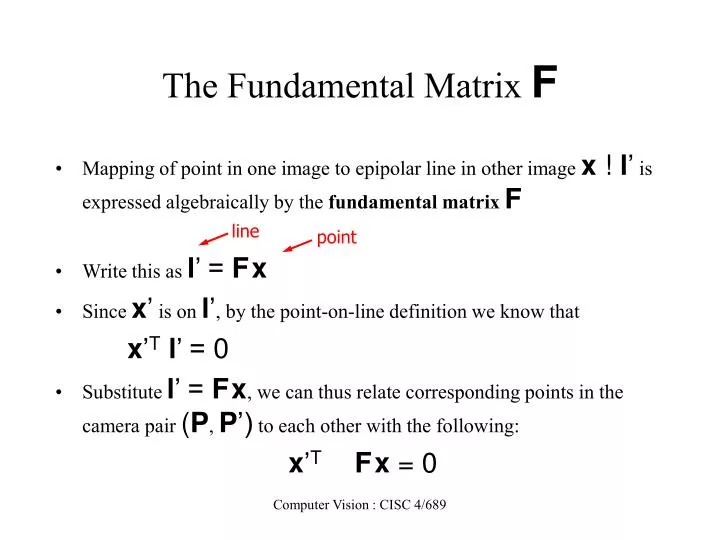
line. point. The Fundamental Matrix F. Mapping of point in one image to epipolar line in other image x ! l ’ is expressed algebraically by the fundamental matrix F Write this as l ’ = F x Since x ’ is on l ’ , by the point-on-line definition we know that x ’ T l ’ = 0

E N D
line point The Fundamental Matrix F • Mapping of point in one image to epipolar line in other image x !l’ is expressed algebraically by the fundamental matrixF • Write this as l’ = Fx • Since x’ is on l’, by the point-on-line definition we know that x’T l’ = 0 • Substitute l’ = Fx, we can thus relate corresponding points in the camera pair (P, P’) to each other with the following: x’T Fx = 0 Computer Vision : CISC 4/689
The fundamental matrix F (courtesy: Marc Pollefeys,UNC) geometric derivation mapping from 2-D to 1-D family (rank 2) Note: rank of skew symmetric matrix is even, so 2, so F’s rank is 2 Computer Vision : CISC 4/689
The Fundamental Matrix F • F is 3 x 3, rank 2 (not invertible, in contrast to homographies) • 7 DOF (homogeneity and rank constraint take away 2 DOF) • The fundamental matrix of (P’, P) is the transpose FT NOW, can get implicit equation for any x, which is epipolar line) x’ Computer Vision : CISC 4/689 from Hartley & Zisserman
Computing Fundamental Matrix (u’ is same as x in the prev. slide, u’ is same as x) Fundamental Matrix is singular with rank 2 In principal F has 7 parameters up to scale and can be estimatedfrom 7 point correspondences Direct Simpler Method requires 8 correspondences Computer Vision : CISC 4/689
The fundamental matrix F (courtesy: Marc Pollefeys,UNC) F is the unique 3x3 rank 2 matrix that satisfies x’TFx=0 for all x↔x’ • Transpose: if F is fundamental matrix for (P,P’), then FT is fundamental matrix for (P’,P) • Epipolar lines: l’=Fx & l=FTx’ • Epipoles: on all epipolar lines, thus e’TFx=0, x e’TF=0, similarly Fe=0 • F has 7 d.o.f. , i.e. 3x3-1(homogeneous)-1(rank2) • F is a correlation, projective mapping from a point x to a line l’=Fx (not a proper correlation, i.e. not invertible) • i.e, mapping is (singular) correlation (projective mapping from points to lines) Computer Vision : CISC 4/689
Estimating Fundamental Matrix The 8-point algorithm Each point correspondence can be expressed as a linear equation Computer Vision : CISC 4/689
The 8-point Algorithm Lot of squares, so numbers have varied range, from say 1000 to 1. So pre-normalize. And RANSaC! Computer Vision : CISC 4/689
Computing F: The Eight-point Algorithm • Input: n point correspondences ( n >= 8) • Construct homogeneous system Ax= 0 from • x = (f11,f12, ,f13, f21,f22,f23 f31,f32, f33) : entries in F • Each correspondence gives one equation • A is a nx9 matrix (in homogenous format) • Obtain estimate F^ by SVD of A • x (up to a scale) is column of V corresponding to the least singular value • Enforce singularity constraint: since Rank (F) = 2 • Compute SVD of F^ • Set the smallest singular value to 0: D -> D’ • Correct estimate of F : • Output: the estimate of the fundamental matrix, F’ • Similarly we can compute E given intrinsic parameters Computer Vision : CISC 4/689
el lies on all the epipolar lines of the left image P Pl Pr True For every pr Epipolar Plane F is not identically zero Epipolar Lines p p r l Ol el er Or Epipoles Locating the Epipoles from F • Input: Fundamental Matrix F • Find the SVD of F • The epipole el is the column of V corresponding to the null singular value (as shown above) • The epipole er is the column of U corresponding to the null singular value • Output: Epipole el and er Computer Vision : CISC 4/689
Special Case: Translation along Optical Axis • Epipoles coincide at focus of expansion • Not the same (in general) as vanishing point of scene lines Computer Vision : CISC 4/689 from Hartley & Zisserman
Finding Correspondences • Epipolar geometry limits where feature in one image can be in the other image • Only have to search along a line Computer Vision : CISC 4/689
Simplest Case • Image planes of cameras are parallel. • Focal points are at same height. • Focal lengths same. • Then, epipolar lines are horizontal scan lines. Computer Vision : CISC 4/689
We can always achieve this geometry with image rectification • Image Reprojection • reproject image planes onto common plane parallel to line between optical centers • Notice, only focal point of camera really matters Computer Vision : CISC 4/689 (Seitz)
P Pl Pr p’ r p’ l Y’l Y’r Z’r Z’l X’l T X’r Ol Or Stereo Rectification • Stereo System with Parallel Optical Axes • Epipoles are at infinity • Horizontal epipolar lines • Rectification • Given a stereo pair, the intrinsic and extrinsic parameters, find the image transformation to achieve a stereo system of horizontal epipolar lines • A simple algorithm: Assuming calibrated stereo cameras Computer Vision : CISC 4/689
P Pl Pr Yr p p r l Yl Xl Zl Zr X’l T Ol Or R, T Xr Xl’ = T_axis, Yl’ = Xl’xZl, Z’l = Xl’xYl’ Stereo Rectification • Algorithm • Rotate both left and right camera so that they share the same X axis : Or-Ol = T • Define a rotation matrix Rrect for the left camera • Rotation Matrix for the right camera is RrectRT • Rotation can be implemented by image transformation Computer Vision : CISC 4/689
P Pl Pr Yr p p r l Yl Xl Zl Zr X’l T Ol Or R, T Xr Xl’ = T_axis, Yl’ = Xl’xZl, Z’l = Xl’xYl’ Stereo Rectification • Algorithm • Rotate both left and right camera so that they share the same X axis : Or-Ol = T • Define a rotation matrix Rrect for the left camera • Rotation Matrix for the right camera is RrectRT • Rotation can be implemented by image transformation Computer Vision : CISC 4/689
P Pl Pr p’ r p’ l Y’l Y’r Zr Z’l X’l T X’r Ol Or R, T T’ = (B, 0, 0), Stereo Rectification • Algorithm • Rotate both left and right camera so that they share the same X axis : Or-Ol = T • Define a rotation matrix Rrect for the left camera • Rotation Matrix for the right camera is RrectRT • Rotation can be implemented by image transformation Computer Vision : CISC 4/689
Public Library, Stereoscopic Looking Room, Chicago, by Phillips, 1923 Computer Vision : CISC 4/689
Teesta suspension bridge-Darjeeling, India Computer Vision : CISC 4/689
Mark Twain at Pool Table", no date, UCR Museum of Photography Computer Vision : CISC 4/689
Woman getting eye exam during immigration procedure at Ellis Island, c. 1905 - 1920, UCR Museum of Phography Computer Vision : CISC 4/689
Stereo matching • attempt to match every pixel • use additional constraints Computer Vision : CISC 4/689
disparity Depth Z Elevation Zw A Simple Stereo System LEFT CAMERA RIGHT CAMERA baseline Right image: target Left image: reference Zw=0 Computer Vision : CISC 4/689
Let’s discuss reconstruction with this geometry before correspondence, because it’s much easier. ( -ve, +ve, refer previous slide fig.) P Similarity of triangles: Xl,f -> X,Z xl,yl=(f X/Z, f Y/Z) Xr,yr=(f (X-T)/Z, f Y/Z) d=xl-xr=f X/Z – f (X-T)/Z Z Disparity: xl xr f pl pr X Ol Or (T-X) But moving to Left camera makes It –(T-X) T Then given Z, we can compute X and Y. T is the stereo baseline d measures the difference in retinal position between corresponding points (Camps) Computer Vision : CISC 4/689
Correspondence: What should we match? • Objects? • Edges? • Pixels? • Collections of pixels? Computer Vision : CISC 4/689
Extracting Structure • The key aspect of epipolar geometry is its linear constraint on where a point in one image can be in the other • By correlation-matching pixels (or features) along epipolar lines and measuring the disparity between them, we can construct a depth map (scene point depth is inversely proportional to disparity) courtesy of P. Debevec View 1 View 2 Computed depth map Computer Vision : CISC 4/689
Correspondence: Photometric constraint • Same world point has same intensity in both images. • Lambertian fronto-parallel • Issues: • Noise • Specularity • Foreshortening Computer Vision : CISC 4/689
For each epipolar line For each pixel in the left image Improvement: match windows Using these constraints we can use matching for stereo • compare with every pixel on same epipolar line in right image • pick pixel with minimum match cost • This will never work, so: (Seitz) Computer Vision : CISC 4/689
Aggregation • Use more than one pixel • Assume neighbors have similar disparities* • Use correlation window containing pixel • Allows to use SSD, ZNCC, etc. Computer Vision : CISC 4/689
? = g f Most popular Comparing Windows: For each window, match to closest window on epipolar line in other image. (Camps) Computer Vision : CISC 4/689
Comparing image regions Compare intensities pixel-by-pixel I(x,y) I´(x,y) Dissimilarity measures • Sum of Square Differences Computer Vision : CISC 4/689
Comparing image regions Compare intensities pixel-by-pixel I(x,y) I´(x,y) Similarity measures Zero-mean Normalized Cross Correlation Computer Vision : CISC 4/689
Small windows disparities similar more ambiguities accurate when correct Large windows larger disp. variation more discriminant often more robust use shiftable windows to deal with discontinuities Aggregation window sizes Computer Vision : CISC 4/689 (Illustration from Pascal Fua)
W = 3 W = 20 Window size • Effect of window size • Better results with adaptive window • T. Kanade and M. Okutomi,A Stereo Matching Algorithm with an Adaptive Window: Theory and Experiment,, Proc. International Conference on Robotics and Automation, 1991. • D. Scharstein and R. Szeliski. Stereo matching with nonlinear diffusion. International Journal of Computer Vision, 28(2):155-174, July 1998 (Seitz) Computer Vision : CISC 4/689
Correspondence Using Window-based matching scanline Right Left SSD error disparity Computer Vision : CISC 4/689 Left Right
Sum of Squared (Pixel) Differences Left Right Computer Vision : CISC 4/689
ImageNormalization • Even when the cameras are identical models, there can be differences in gain and sensitivity. • The cameras do not see exactly the same surfaces, so their overall light levels can differ. • For these reasons and more, it is a good idea to normalize the pixels in each window: Computer Vision : CISC 4/689
Stereo results • Data from University of Tsukuba Scene Ground truth (Seitz) Computer Vision : CISC 4/689
Results with window correlation Window-based matching (best window size) Ground truth (Seitz) Computer Vision : CISC 4/689
Results with better method • State of the art method • Boykov et al., Fast Approximate Energy Minimization via Graph Cuts, • International Conference on Computer Vision, September 1999. Ground truth Computer Vision : CISC 4/689 (Seitz)