Download
1 / 48
550 likes | 1.79k Vues
PID Control System Analysis and Design. Presented by Binu Mammen Noah Berhanu Souvik Bhattacharya Vishal Raj Karunala. Introduction. Proportional-integral-derivative (PID) control provides a generic and efficient solution to real world control problems

E N D
PID Control SystemAnalysis and Design Presented by Binu Mammen Noah Berhanu Souvik Bhattacharya Vishal Raj Karunala
Introduction • Proportional-integral-derivative (PID) control provides a generic and efficient solution to real world control problems • Presents remedies for problems involving the integral and derivative terms. PID design objectives,methods, and future directions are discussed.
What is PID • PID stands for Proportional, Integral, Derivative. Controllers are designed to eliminate the need for continuous operator attention. • Cruise control in a car and a house thermostat are common examples • Error is defined as the difference between set-point and measurement. (error) = (set-point) - (measurement) • The output of PID controller will change in response to the error
What IS PID Proportional • With proportional band, the controller output is proportional to the error or a change in measurement. • (controller output) = (error)*100/(proportional band) • Drawbacks -With a proportional controller offset is present. • Increasing the controller gain will make the loop go unstable. • Integral action was included in controllers to eliminate this offset
What IS PID Integral • With integral action, the controller output is proportional to the amount of time the error is present. Integral action eliminates offset. • Controller Output = (1/INTEGRAL) (Integral of)e(t)d(t) • Integral action gives the controller a large gain at low frequencies
What IS PID Derivative • The controller output is proportional to the rate of change of the measurement or error • CONTROLLER OUTPUT = DERIVATIVE - dm/dt
STANDARD STRUCTURES OF PID CONTROLLERS Parallel Structure and Three-Term Functionality • T.F-: GPID(s) =U(s)/E(s) = KP(1 +1/T1s + TDs)…..(1) U(s) is the control signal E(s)=Error signal. constant, TD =Derivative time constant TI =Integral time constant S=Argument of the Laplace transform. • Control Signal can be expressed in three terms as • U(s) = KPE(s) + KI1/sE(s) + KDsE(s) • U(s) = UP(s) + UI(s) + UD(s),
STANDARD STRUCTURES OF PID CONTROLLERS Parallel Structure and Three-Term Functionality • Where KI = KP/TI is the integral gain and KD = KPTD is the derivative gain. The three-term functionalities include: • The proportional term provides an overall control action proportional to the error signal through the all pass gain factor. • The integral term reduces steady-state errors through low-frequency compensation. • The derivative term improves transient response through High-frequency compensation.
STANDARD STRUCTURES OF PID CONTROLLERS • A PID controller is a phase lead-lag compensator with one pole at the origin and the other at infinity. • PI-Phase lag. • PD-Phase-lead compensators. • Optimum perfomance can be achieved Kp KI Kd are tuned together
STANDARD STRUCTURES OF PID CONTROLLERSSeries Structure • GPID(s) = (α + TDs) KP (1 +1/αT1s)…………..(3) • GPID(s)=GPD(s)GPI(s) • GPD(s)GPI(s) are the factored PD and PI parts
Adding an integral term to a pure proportional term increases the gain by a factor. Increases the phase-lag Gain margin (GM) and phase margin (PM) are reduced, and the closed-loop system becomes more oscillatory and potentially unstable Integral TermDestabilizing Effect of the Integral Term
Integrator Windup • If the actuator realizes the control action has saturated range limits, and the saturations are neglected in a linear control design, the integrator may suffer from windup; this causes low-frequency oscillations and leads to instability • Windup is due to the controller states becoming inconsistent with the saturated control signal, and future correction is ignored until the actuator desaturates
Integrator Windup Remedies • Antiwindup can be achieved implicitly through automatic reset. • Explicit Antiwindup implemented explicitly through internal negative feedback. • Another Solution to antiwindup is to reduce the possibilities for saturation by reducing the control signal, as in linear quadratic optimal control schemes that minimize the tracking error and control signal through a weighted objective function.
Integral TermDestabilizing Effect of the Integral Term • UI(s) =1/TIs (KPE(s) −U(s) −Ucap(s)/ r(gamma),
Contents • General form and uses • Drawbacks • Remedies
General form • PD = ( 1 + Tds ) • Frequency response = ( 1 + jwTd) • Gain = | 1 + jwTd|
Uses • Improved damping ratio • Fast recovery from disturbance • Strong signal for error signal
Drawbacks an example • G = (Ke-Ls) / ( 1 + T s ) • | G (jw)Gpd(jw) | > 1 for all w if Kp > 1/K and Td > T / K Kp • tan -1 ( wTd) tan-1 (Tw) – Lw phase angle < -180 • Unstable system
Remedies • Involves use of filters • Linear low pass filter • Velocity Feedback • SetPoint Filter • Nonlinear median filter
Linear low pass filter • Second order Butterworth filter Gd (s) = KpTd s / ( 1 + Td/ bs ) • Value of b [ 8,16 ] • Cascaded to the PD only or to the whole PID controller ( slow transient response)
e + Kp (.) + Ki ∫ (. ) G(s) + - - Kd d( . ) dt Velocity feedback • Known as PI-D or Type B controller • PD placed in the feedback + Y
Set point filter • Known also as P-ID or Type C controller • Similar to Type B • Gives good overshot performance for a good choice of b - Kp b + e + G(s) y + r Ki ∫ ( . ) + - - Kd d ( . ) dt
Median filter • Often used in DIP • Setting the current value to the median values of nearby data points • Removes spikes drawback • Excessive smoothness for under damped system
DESIGN OBJECTIVES AND EXISTING METHODS • Matters concerning commission and maintenance(such as pre- and post-processing as well as fault tolerance) also need to be considered in a complete PID design. • Controller parameters are tuned so that so that the closed loop system meets the following five objectives: • stability and stability robustness, usually measured in the frequency domain. • transient response, including rise time, overshoot, and settling time. • steady-state accuracy.
……..CONTD 4. disturbance attenuation and robustness against environmental uncertainty, often at steady state 5. robustness against plant modeling uncertainty, usually measured in the frequency domain. • Most methods target one objective or a weighted composite of the objectives listed above.
Heuristic Methods • Heuristic methods evolve from empirical tuning (such as the ZN tuning rule), often with a tradeoff among design objectives. Heuristic search involves expert systems, fuzzy logic, neural networks, and evolutionary computation
Frequency-domain constraints, such as GM, PM, and sensitivities, are used to synthesize PID controllers offline. For real-time applications, frequency-domain measurements require time-frequency, localization-based methods such as wavelets. Frequency Response Methods
Analytical Methods • Because of the simplicity of PID control, parameters can be derived analytically using algebraic relations between a plant model and a targeted closed-loop transfer function with an indirect performance objective, such as pole placement, IMC, or lambda tuning
Numerical Optimization Methods • Optimization-based methods can be regarded as a special type of optimal control. • PID parameters are obtained by numerical optimization for a weighted objective in the time domain. • a self-learning evolutionary algorithm (EA) can also be used to search for both the parameters and their associated structure or to meet multiple design objectives in both the time and frequency domains • These designs are suitable for adaptive tuning as some of the designs can be computerized ,so that are automatically performed online once the plant is identified. • most widely adopted initial tuning methods are based on the Z-N empirical formulas and their extensions.
Computerized Simulation Approach • By using a computerized approach, multiple design methods can be combined within a single software or firmware package to support various plant types and PID structures. • PIDeasy is a software package that uses automatic simulations to search globally for controllers that meet all five design objectives in both the time and frequency domains.
First-Order Delayed Plants • While requirements of fast transient response, no overshoot,and zero steady-state error are accommodated by timedomain criteria, PIDeasy’s multiobjective goals provide frequency-domain margins in the range of 9–11 dB and 65–66 degrees. • To assess the robustness of design using PIDeasy, GMs and PMs resulting from designs for plants with various L/T ratios are shown in the figure.
SETPOINT-SCHEDULED PID NETWORK • Consider the constant-temperature reaction process where y(t) = concentration in the outlet stream (mol/l), u(t) = flow rate of the feed stream (l/h), K = rate of reaction (l/mol-h), V = reactor volume (l), d = concentration in the inlet stream (mol/l).
The set point, equilibrium, or steady-state operating trajectory of the plant is governed by • Placement at y=0.49 using the maximum distance from the nonlinear trajectory to the linear projection linking the starting and ending points of the operating envelope.
Obtaining the individual PID controllers by using PIDeasy or other PID software or jointly by an evolutionary algorithm, without linearization.
Addition of two more controllers at nodes or setpoints 1 and 3. • Formation of a pseudo-linear controller network comprised of three PIDs to be interweighted by scheduling functions S1(y), S2(y), and S3(y).
Due to nonlinearity, these functions are often asymmetric. • Similar to gain scheduling, linear interpolation meets the requirements for setpoint scheduling.
The resulting PID network is given by where p denotes the derivative operator.
Performance of the pseudo-linear PID network applied to the nonlinear process example.
To validate tracking performance, another setpoint r = 0.53 mol/l is used to test the control system. • The controller network tracks this setpoint change accurately without oscillation. • A 10% load disturbance occurring during [3, 3.5] h,is rejected confirming load disturbance rejection at steady state.
SUMMARY • What is PID? PID Controller stands for Proportional-Integral-Derivative Controller. It is a type of feedback controller. It can also be referred to as the “Tuner”. • Why should we use the PID controller? 1. The Controller provides the excitation for the plant. 2. Designed to control the overall system behavior. • What is Tuning? Tuning is nothing but the individual adjustment of the proportional, integral and derivative terms. • What exactly does it do? It helps to achieve the output (velocity, temperature, position) desired, in a short time, with minimal overshoot, and with little error.
PID equation Kp – Proportional Gain Ki – Integral Gain Kd- Derivative Gain EXAMPLES: • A motor driving a gear train • A thermal system - A Heater • Mechanical Devices.
DRAWBACKS: • PID control can be costly to implement and support. • It requires frequent valve- and damper-position readjustment and this nearly continuous repositioning shortens actuator life, adds to maintenance costs, and makes control stability a question.
ENHANCEMENT: • NEWPORT MICRO-INFINITY®: Most sophisticated form of discrete control available today. • The NEWPORT MICRO-INFINITY® is a full function “Auto tune” (or self-tuning) PID controller which combines proportional control with two additional adjustments, which help the unit automatically compensate to changes in the system. • These adjustments, integral and derivative, are expressed in time-based units.
CONCLUSIONS: • Cost effectiveness: Division of self-contained stand-alone instructional units around standard PID structures. • Automation by including system identification techniques and modular code blocks can be made available for timely application and adaptation in real-time.