Download
1 / 47
570 likes | 884 Vues
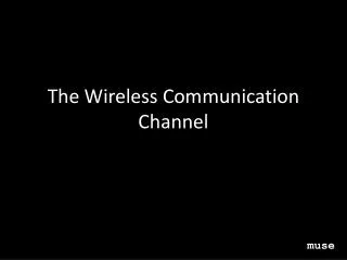
The Wireless Channel. Shivkumar Kalyanaraman shivkumar-k AT in DOT ibm DOT com http://www.shivkumar.org Google: “shivkumar ibm rpi”. Slides based upon books by Tse/Viswanath, Goldsmith, Rappaport, J.Andrews etal . Wireless Channel is Very Different!.

E N D
The Wireless Channel Shivkumar Kalyanaraman shivkumar-k AT in DOT ibm DOT com http://www.shivkumar.org Google: “shivkumar ibm rpi” Slides based upon books by Tse/Viswanath, Goldsmith, Rappaport, J.Andrews etal
Wireless Channel is Very Different! • Wireless channel “feels” very different from a wired channel. • Not a point-to-point link • Variable capacity, errors, delays • Capacity is shared with interferers • Characteristics of the channel appear to change randomly with time, which makes it difficult to design reliable systems with guaranteed performance. • Cellular model vs reality: Cellular system designs are interference-limited, i.e. the interference dominates the noise floor
Basic Ideas: Path Loss, Shadowing, Fading • Variable decay of signal due to environment, multipaths, mobility Source: A. Goldsmith book
Small-Scale Fading: Multipath (frequency domain) & Mobility (time-domain) Channel varies at two spatial scales: * Large scale fading: path loss, shadowing * Small scale fading: Multi-path fading (frequency selectivity, coherence b/w, ~500kHz), Doppler (time-selectivity, coherence time, ~2.5ms)
Effect of Multipath fading: Attenuation, Dispersion leading to ISI! Inter-symbol interference (ISI) Source: Prof. Raj Jain, WUSTL
Large-scale Fading: Path Loss, Shadowing More important for cell site planning, less for communication system design.
Free-Space-Propagation • If oscillating field at transmitter, it produces three components: • The electrostatic and inductive fields that decay as 1/d2 or 1/d3 • The EM radiation field that decays as 1/d (power decays as 1/d2)
Simplified Path Loss Model • Used when path loss dominated by reflections. • Most important parameter is the path loss exponent g, determined empirically. • Cell design impact: If the radius of a cell is reduced by half when the propagation path loss exponent is 4, the transmit power level of a base station is reduced by 12dB (=10 log 16 dB). • Costs: More base stations, frequent handoffs
Typical large-scale path loss Source: Rappaport and A. Goldsmith books
Path Loss Effects: Carrier Frequency • Note: effect of frequency f: 900 Mhz vs 5 Ghz. • Either the receiver must have greater sensitivity or the sender must pour 44W of power, even for 10m cell radius! 10m W Source: A. Goldsmith book
Path Loss: Interference & Cell Sizing • Desired signal power: • Interference power: • SIR: • SIR is much better with higher path loss exponent ( = 5)! • Higher path loss, smaller cells => lower interference, higher SIR Source: J. Andrews et al book
Critical Distance & cell size design • Design the cell size to be < critical distance to get: • O(d-2) power decay in cell and… • O(d-4) power decay outside the cell! • Cell radii are typically much smaller than critical distance Source: A. Goldsmith book
Path Loss: Range vs Bandwidth Tradeoff • Frequencies < 1 GHz are often referred to as “beachfront” spectrum. Why? • 1. High frequency RF electronics have traditionally been harder to design and manufacture, and hence more expensive. [less so nowadays] • 2.Pathloss increases ~ O(fc2) • A signal at 3.5 GHz (one of WiMAX’s candidate frequencies) will be received with about 20 times less power than at 800 MHz (a popular cellular frequency). • Effective path loss exponent also increases at higher frequencies, due to increased absorption and attenuation of high frequency signals • Tradeoff: • Bandwidth at higher carrier frequencies is more plentiful and less expensive. • Does not support large transmission ranges. • (also increases problems for mobility/Doppler effects etc) • Broadband Wireless Choice: • Pick any two out of three: high data rate, high range, low cost.
Empirical Models • Okumura model • Empirically based (site/freq specific) • Awkward (uses graphs) • Hata model • Analytical approximation to Okumura model • Cost 136 Model: • Extends Hata model to higher frequency (2 GHz) • Walfish/Bertoni: • Cost 136 extension to include diffraction from rooftops Commonly used in cellular system simulations
Empirical Path Loss: Okamura, Hata, COST231 • Empirical models include effects of path loss, shadowing and multipath. • Multipath effects are averaged over several wavelengths: local mean attenuation (LMA) • Empirical path loss for a given environment is the average of LMA at a distance d over all measurements • Okamura: based upon Tokyo measurements. 1-100 lm, 150-1500MHz, base station heights (30-100m), median attenuation over free-space-loss, 10-14dB standard deviation. • Hata: closed form version of Okamura • COST 231: Extensions to 2 GHz Source: A. Goldsmith book
Indoor Models • 900 MHz: 10-20dB attenuation for 1-floor, 6-10dB/floor for next few floors (and frequency dependent) • Partition loss each time depending upton material (see table) • Outdoor-to-indoor: building penetration loss (8-20 dB), decreases by 1.4dB/floor for higher floors. (reduced clutter) • Windows: 6dB less loss than walls (if not lead lined)
Shadowing • Log-normal model for shadowing r.v. ()
Log-Normal Shadowing • Assumption: shadowing is dominated by the attenuation from blocking objects. • Attenuation of for depth d: s(d) = e−αd, (α: attenuation constant). • Many objects: s(dt) = e−α∑ di= e−αdt , dt= ∑ diis the sum of the random object depths • Cental Limit Theorem (CLT): αdt = log s(dt) ~ N(μ, σ). • log s(dt) is therefore log-normal
dBm Outage Probability: Path Loss & Shadowing • Need to improve receiver sensitivity (i.e. reduce Pmin) for better coverage.
Shadowing: Adaptive Modulation Design • Simple path loss/shadowing model: • Find Pr: • Find Noise power:
Shadowing: Adaptive Modulation Design • SINR: • Without shadowing ( = 0), BPSK works 100%, 16QAM fails all the time. • With shadowing (s= 6dB): BPSK: 16 QAM • 75% of users can use BPSK modulation and hence get a PHY data rate of 10 MHz · 1 bit/symbol ·1/2 = 5 Mbps • Less than 1% of users can reliably use 16QAM (4 bits/symbol) for a more desirable data rate of 20 Mbps. • Interestingly for BPSK, w/o shadowing, we had 100%; and 16QAM: 0%!
Path Loss Models: Summary • Path loss models simplify Maxwell’s equations • Models vary in complexity and accuracy • Power falloff with distance is proportional to d2 in free space, d4 in two path model • General ray tracing computationally complex • Empirical models used in 2G/3G/4G simulations • Main characteristics of path loss captured in simple model Pr=PtK[d0/d]g • Shadowing modeled as log-normal allows the use of adaptive modulation; but complicates cell-site design
Small-Scale Fading: Rayleigh/Ricean Models,Multipath & Doppler
Small-scale Multipath fading: System Design • Wireless communication typically happens at very high carrier frequency. (eg. fc = 900 MHz or 1.9 GHz for cellular) • Multipath fading due to constructive and destructive “self” interference of the transmitted waves. • Channel varies when mobile moves a distance of the order of the carrier wavelength. This is about 0.3 m for 900 Mhz cellular. • For vehicular speeds, this translates to channel variation of the order of 100 Hz. • Primary driver behind wireless communication system design.
#1: Single-Tap (Narrow-Band) Channel: Rayleigh Dist’n • Path loss, shadowing => average signal power loss • Fading around this average. • Subtract out average => fading modeled as a zero-mean random process • Narrowband Fading channel: Each symbol is long in time • The channel h(t) is assumed to be uncorrelated across symbols => single “tap” in time domain. • Fading w/ many scatterers: Central Limit Theorem • In-phase (cosine) and quadrature (sine) components of the snapshot r(0), denoted as rI (0) and rQ(0) are independent Gaussian random variables. • Envelope Amplitude: • Received Power:
Normal Vector R.V, Rayleigh, Chi-Squared X = [X1, …, Xn] is Normal random vector ||X|| is Rayleigh { eg: magnitude of a complex gaussian channel X1 + jX2 } ||X||2 is Chi-Squared w/ n-degrees of freedom When n = 2, chi-squared becomes exponential. {eg: power in complex gaussian channel: sum of squares…}
path-1 Power path-2 path-3 path-2 Path Delay path-1 path-3 Channel Impulse Response: Channel amplitude |h| correlated at delays . Each “tap” value @ kTs Rayleigh distributed (actually the sum of several sub-paths) #2: Broadband / Multipath Channel: Power-Delay Profile (PDP) multi-path propagation Mobile Station (MS) Base Station (BS)
Multipath: Time-Dispersion => Frequency Selectivity • The impulse response of the channel is correlated in the time-domain (sum of “echoes”) • Manifests as a power-delay profile, dispersion in channel autocorrelation function A() • Equivalent to “selectivity” or “deep fades” in the frequency domain • Delay spread: ~ 50ns (indoor) – 1s (outdoor/cellular). • Coherence Bandwidth: Bc = 500kHz (outdoor/cellular) – 20MHz (indoor) • Implications: High data rate: symbol smears onto the adjacent ones (ISI). Multipath effects ~ O(1s)
Set of multipaths changes ~ O(5 ms) #3: Doppler: Time-varying Non-Stationary Channel.
Doppler: Dispersion (Frequency) => Time-Selectivity • The doppler power spectrum shows dispersion/flatness ~ doppler spread (100-200 Hz for vehicular speeds) • Equivalent to “selectivity” or “deep fades” in the time domain correlation envelope. • Each envelope point in time-domain is drawn from Rayleigh distribution. But because of Doppler, it is not IID, but correlated for a time period ~ Tc (correlation time). • Doppler Spread: Ds ~ 100 Hz (vehicular speeds @ 1GHz) • Coherence Time: Tc = 2.5-5ms. • Implications: A deep fade on a tone can persist for 2.5-5 ms! Closed-loop estimation is valid only for 2.5-5 ms.
Fading Summary: Time-Varying Channel Impulse Response • #1: At each tap, channel gain |h| is a Rayleigh distributed r.v.. The random process is not IID. • #2: Response spreads out in the time-domain (), leading to inter-symbol interference and deep fades in the frequency domain: “frequency-selectivity” caused by multi-path fading • #3: Response completely vanish (deep fade) for certain values of t: “Time-selectivity” caused by doppler effects (frequency-domain dispersion/spreading)
Fading: Jargon • Flat fading: no multipath ISI effects. • Eg: narrowband, indoors • Frequency-selective fading: multipath ISI effects. • Eg: broadband, outdoor. • Slow fading: no doppler effects. • Eg: indoor Wifi home networking • Fast Fading: doppler effects, time-selective channel • Eg: cellular, vehicular • Broadband cellular + vehicular => Fast + frequency-selective
Rayleigh Fading Example • Non-trivial (1%) probability of very deep fades. • These very deep fades occur often enough to dominate system performance
Rayleigh Fading (Fade Duration Example) Lz: Level Crossing Rate Faster motion & doppler better (get out of fades)!
Power Path Delay path-1 path-2 path-3 No Symbol Error! (~kbps) (energy is collected over the full symbol period for detection) Delay spread ~ 1 s Symbol Error! If symbol rate ~ Mbps Power Delay Profile => Inter-Symbol interference Symbol Time Symbol Time • Higher bandwidth => higher symbol rate, and smaller time per-symbol • Lower symbol rate, more time, energy per-symbol • If the delay spread is longer than the symbol-duration, symbols will “smear” onto adjacent symbols and cause symbol errors OFDM: Uses a number of “sub-carriers” to ensure “flat fading” in each sub-carrier
Multipaths & Bandwidth (Contd) • Even though many paths with different delays exist (corresponding to finer-scale bumps in h(t))… • Smaller bandwidth => fewer channel taps (remember Nyquist?) • The receiver will simply not sample several multipaths, and interpolate what it does sample => smoother envelope h(t) • The power in these multipaths cannot be combined! • In CDMA Rake (Equalization) Receiver, the power on multipath taps is received (“rake fingers”), gain adjusted and combined. • Similar to bandpass vs matched filtering (see next slide)
Matched Filter: includes more signal power, weighted according to size => maximal noise rejection & signal power aggregation! Rake Equalization Analogy: Bandpass vs Matched Filtering Simple Bandpass (low bandwidth) Filter: excludes noise, but misses some signal power in other mpath “taps”