Download
1 / 24
250 likes | 579 Vues
T Tests: Comparison of Means. Most t tests involve the comparison of two populations with respect to the means of randomly drawn samples from the respective populations.

E N D
T Tests: Comparison of Means • Most t tests involve the comparison of two populations with respect to the means of randomly drawn samples from the respective populations. • The two populations could be different groups or experimental conditions, or they could be “within” persons or units, such as a “before” and “after” design, e.g., the population of people who were tested before a treatment and the population of people who were tested after it • If the obtained scores within a sample are reasonably homogeneous (have low variability), and the variances of the two groups are roughly equal, then a difference of means test is an appropriate way to test hypotheses about the differences between two populations
T-Test and The Null Hypothesis • The null hypothesis, usually expressed as µ1 = µ2 , is what we ordinarily seek to reject (but sometimes fail to reject) in statistical hypothesis testing • With respect to the difference of means test, the null hypothesis is that any differences we observe in the samples we draw from the two populations were obtained by chance (due to sampling error), and that the differences in the population means are zero • If the observed differences we obtain in our samples are not sufficiently large (don’t fall within the predetermined confidence region), we can say that we have failed to reject the null hypothesis or alternatively that we must retain the null hypothesis
T Test and the Research Hypothesis • The research hypothesis, µ1 ≠ µ2 , is that the population means are unequal, i.e., that there are differences between the populations. When we get a result such that we can reject the null hypothesis, we then can certainly say that there is evidence to support the research hypothesis. Some researchers will state this as “confirming” or “accepting” the research hypothesis
Sampling Distribution of Differences between Means • Underlying the t statistic is the notion of a sampling distribution of differences between means • In this distribution it is assumed that any obtained differences between pairs of samples (say, samples of males and females, or befores and afters) are due to sampling error and do not represent true population differences • The sampling distribution of differences between means approximates a normal distribution with a mean of zero for samples over size 100
Formula for t • In this formulat, the expression in the numerator is the difference between the obtained sample means for the two groups (treatments, etc) we are comparing and in the denominator we have an estimate of the standard deviation of the sampling distribution of the differences between sample means. We estimate this denominator based on sample values (more on how to calculate this in a minute).
Significance Levels • Significance levels, also known as confidence levels, critical values, rejection levels (for the null hypothesis), alpha levels, etc: they are the points at which the region beyond them under the curve (of the test statistic distribution) contains such unlikely occurrences that, when an obtained sample value falls into that region, one can reject the null hypothesis with confidence • It is conventional to set the confidence level in advance of performing the test to .05 (two-tailed, which means that the obtained statistic has to fall into one of the two regions which represent the upper and lower .025 of the area under the curve) for non-critical applications and to more stringent levels like .001 or .0001 for medical or other critical applications
Setting Significance Levels • The researcher will opt for a one-tailed test whenever s/he is able to predict the direction of differences. This means that a result must be obtained that falls within the upper 5% of the area under the curve, or the lower 5%, depending upon the predicted direction of the differences • Most of the research you will do will not require that you set a significance level higher than .05, one-tailed • Most risk of Type II error (failing to reject the null hypothesis when it is in fact false) can be avoided if you have sufficiently large samples • Distinction between P and alpha: P is the exactly probability level associated with an obtained statistics such as a t score and is gotten from the raw data. SPSS will give you this value. Alpha level refers to the size of the critical region under the curve into which our test statistic must fall, according to our requirements. • SPSS will automatically calculate the actual probability for you. You may report this value in a research report, but you will base your decision about whether or not to reject the null hypothesis based on whether or not your obtained value of t, is greater than the value of t associated with the confidence level you set in advance
Further Criteria for Setting Significance Levels • Plausibility of alternatives: if the research hypothesis is directly counter to prevailing theory, it is better to set a more stringent level than .05 • Sample size: when the sample size is small, the power to detect an effect is less, so the critical region should be more generous • Degree of control in experimental design: the greater the degree of control (e.g. the more extraneous influences eliminated which could account for the observed variation between conditions of the experiment) the greater the freedom to use a larger critical region to detect an effect • Extent to which data do not meet assumptions of the statistical test (independence of cases, random sampling, equality of variances, etc): when data do not meet assumptions of statistical test better to use a smaller error rate such as .025 and interpret it as a larger one • Direction of hypothesis: should choose a smaller critical region if you are confident of the direction of the difference of means, etc. • Testing vs. developing hypotheses: A larger confidence region can be used for pilot studies.
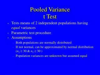
T test for Independent or Unmatched Samples • The purpose of the t test is to make a determination with respect to two sample means whether or not they were drawn from different populations. Another way to put this is to decide if the means for the two samples (two samples which differ on the “grouping variable” )“differ significantly” on the variable of interest (the “test variable”) • There are several varieties of t test • Most generally, the t test assumes that the standard deviations σ1 and σ2 in the two populations are equal (we can call this Model A). • However, there are times when we would not make this assumption (we will call this Model B; σ1 ≠ σ2 ) (When conducting a t test in SPSS for independent samples, the program will conduct a test for homogeneity of variance and give you values of t assuming both models A and B)
T test for Independent or Unmatched Samples, cont’d • Use of t test assumes that the populations from which the samples are drawn are normally distributed with respect to the variables of interest • Use of t test assumes interval level data (minimally) and random sampling • Sometimes referred to as a Z-test since t is normally distributed for large samples. In fact for n > 120 it is OK to consult the Z table to obtain the probability • The obtained value of t and its significancedepend on (1) the size of the mean differences (2) the amount of variability within each sample (3) the sample size • Small variability and large sample size give us more confidence in the results we obtain
Model A t test: Equal Population Variances are Assumed • Let’s consider an example of Model A, when we make the assumption that the variances in the populations are equal. We have the following problem: • In a study of attitudes toward smoking, it was found than an experimental group (N=40, s = 6) who had visited a Web site organized by the Tobacco Lobbyist’s League had a mean score on the “smoking favorability” test of 40, while a control group (N = 22, s = 4) had a mean score on the smoking favorability test of 35. Higher scores on the test reflect greater favorability towards smoking • Our null hypothesis, H0, is that the two groups are from the same population • Our research hypothesis, H1, is that the two groups are from different populations. Another way to put this is that we hypothesize that the two groups differently significantly with respect to the variable of interest, scores on the smoking favorability test. Further, we anticipate that the differences will be such that that experimental group will have a higher mean than the control group on the smoking favorability test, so we have a predicted direction of differences
Model A t test, Equal Variances, cont’d • To test the null hypothesis we will turn to the t test. • We will make a decision that to reject the null hypothesis we will require a value of t that falls into the p <.05 critical region of the t distribution, and that this will be a one-tailed test, since we have hypothesized a particular direction of differences (that the mean for the Experimental Group will be greater than the mean for the Control Group). A smaller value of t is required for the same level of significance with a one-tailed test (e.g., t might be significant at the .05 level with a one-tailed test, but only at the .10 level for a two-tailed test) • Our DF to enter the t table is N1 + N2-2, or 60. • To reject the null hypothesis with DF = 60 we need a value of t of 1.671 for a one-tailed test (see next slide)
Calculation of Test Statistic for Pooled Variance t Test, Model A (Equal Variances Assumed) • How is t calculated when it is assumed that the population variances for the two groups are equal? • Recall that the experimental Group (N=40, s = 6) who had visited a Web site organized by the Tobacco Lobbyist’s League had a mean score on the “smoking favorability” test of 40, while a control group (N = 22, s = 4) had a mean score on the smoking favorability test of 35. • The numerator in the “real” formula for t is the difference of the two sample means minus the difference of the populations means. However, under the null hypothesis, the population means are assumed to be equal and the second term (zero) drops out, so the numerator of t is just the difference between the means of the two groups. In our case, that is +5. (40-35) • In calculating the denominator, we want to have some measure of the variance of the sampling distribution of the differences in sample means. Because of the assumption of equal population variances, we are going to use a “pooled estimate.” To calculate the denominator, we first have to find the “weighted average of variances.”We will symbolize this pooled denominator as sp2
Computing the Weighted Average of Variances for the Denominator of the t Statistic, Model A • To compute the pooled, weighted average of variances, we need to assemble our sample data: N1 = 40, N2 = 22, M1 = 40, M2 = 35, s1 = 6, s2 = 4. The weighted average of variances, sp2, equals (N1-1)S12 + (N2-1)S22 (N1 + N2) - 2 Inserting our sample data into the formula, we have (39)(36) + (21)(16) / 40 + 22 -2 = 1404 + 336/60 = 29. Thus sp2 equals 29.
Calculation of t, Model A (Equal Variances Assumed) • Calculate t: Pooled estimate of the standard deviation of the sampling distribution of differences in sample means is in the denominator-what we computed on previous slide X1 – X2 t = √sp2 N1 + Sp2 N2 The numerator of t equals the mean of group 1 (40) minus mean of group 2 (35) or 5. This value, 5, is divided by the square root of (29/40 + 29/22) and t equals 3. 498. Can we reject the null hypothesis? In other words, how likely is it that we would obtain a value of t as large as 3.498 if the experimental and control groups were from the same population with respect to the variable of interest? Looking up in the table we find that a t of 3.498 is significant (p < .005, one-tailed, DF = 60) and we can reject the null hypothesis-can say that the experimental and control groups differ significantly.
Model B, Equal Population Variances Not Assumed (t-test for Unequal Variances) • If we cannot assume equal variations in the populations from which the samples are purportedly drawn, then we need a different estimate of the standard error of the sampling distribution of differences of means in the denominator • In calculating t we use almost the same formula as in the previous model but instead we substitute the separate sample variances for the pooled or weighted average of variances, sp2, that we used in the first model So in this case , t would be equal to 5/ the square root of 36/40 + 16/22, or 3.919. This statistic requires that you compute a different DF before consulting the t distribution table Some authorities, like Blalock, use N1-1 and N2 -2 in the denominator for unequal variances. X1 – X2 √s12 N1 + S22 N2
Using SPSS to conduct a t Test for Independent Samples, Assuming Equal Population Variances • Let’s use the data from the employment2.sav data file to test the research hypothesis that males and females differed with respect to how long they had been at their current job at the time of data collection. The null hypothesis would be that with respect to the variable “months of experience at the current job” men and women are from the same population • In SPSS go to Analyze/Compare Means/Independent Samples t-tests • Move the Previous Experience variable into the Test Variable box and move Gender into the Grouping box. Click on the Define Groups button (if it is blanked out highlight the variable name in the box above it) and define the first group as “1” and the second group as “2,” and click Continue • Under Options, set the confidence interval to 95%, click Continue and then OK • Compare your output to the next slide
SPSS Output, t Test for Independent Samples with both Equal and Unequal Variances Assumed Can we reject the null hypothesis that there are no differences between males and females in months of previous experience?
T test for Dependent or Matched Samples • In certain cases, for example in “before and after” designs or when members of group A have been matched with members of group B on all salient characteristics except one, the variable of interest, an alternative formula for computing t is used. For example, you might want to find out if there have been significant changes in brand preference among the same persons following exposure to a commercial • In this type of t test, we treat a “pair” of individuals as a case, rather than the N1 + N2 individuals we ordinarily treat as cases • We test a hypothesis of the following form: the mean of the pair-by-pair differences in the population, µD , is zero; in this case, that there are no differences attributable to exposure to the commercial
An Example of t-Test for Dependent Samples • Problem: Ten subjects are given a pre-test on attitudes toward downloading of “hijacked” movie files. They heard a commercial from a union representing technical people in the motion picture industry in which they talked about having people “steal” the fruits of their labors. The ten people then were re-administered the attitude measure. Given the pre- and post-test scores below, can you conclude, at the p <.01 level, one-tailed, that the commercial made a significant impact on attitudes toward movie downloading? (Higher scores on the test mean more negative attitudes toward downloading) Where XD-bar is the mean difference between pairs of scores, N is the # of pairs of scores, the XD are the differences between each of the matched pairs of scores t =XD √∑(XD –XD)2 / √(N-1) N Note: this computing formula gives an equivalent result to pp. 152-154 in Levin and Fox
Calculation of t for dependent Samples Calculate t for this data: XD = 5; ∑(XD –XD)2 = 354, N= 10, DF=N-1 t = 5 √(354/10) /√9 = 5/1.983 = 2.521 Mean difference in positivity after hearing a commercial against pirating movie files
T Test for Dependent Samples in SPSS • Now let’s try that in SPSS. Go here to download the pre/post data set • In SPSS Data Editor, go to Analyze/Compare Means/ Paired Sample • Put the Posttest and Pretest variables into the Paired Variables box; put Posttest in first if you expect posttest scores to be higher • Click Options and select the 95% confidence interval, and click Continue, then click OK • Compare your results to your hand calculations
Output for Paired Samples t Test Note that the mean is higher (e.g. in this case a more positive attitude) after the commercial This correlation indicates that about 49% (1-(.692)2)of the variation in post-test attitudes could be explained by pre-test attitudes. Presumably the rest of the variation is explained by treatment plus error We have a significant value of t, but look at that confidence interval ;-( Also, compare the means; does this seem like a major change? And compare the standard deviations; in both cases they are all over the place in the raw scores So we can reject the null hypothesis of no differences between pre and post and conclude that our treatment increased negative attitudes towards downloading