Download
1 / 27
270 likes | 381 Vues
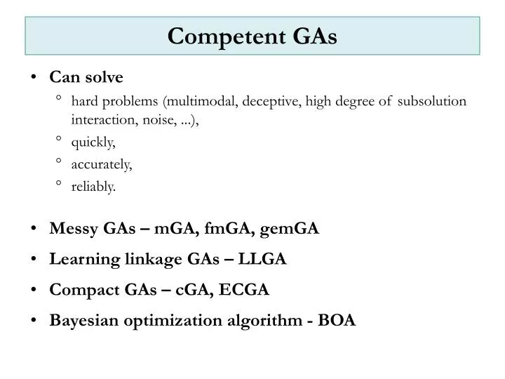
Competent GAs. Can solve hard problems (multimodal, deceptive, high degree of subsolution interaction, noise, ...), quickly, accurately, reliably. Messy GAs – mGA, fmGA, gemGA Learning linkage GAs – LLGA Compact GAs – cGA, ECGA Bayesian optimization algorithm - BOA. Messy GAs.

E N D
Competent GAs • Can solve • hard problems (multimodal, deceptive, high degree of subsolution interaction, noise, ...), • quickly, • accurately, • reliably. • Messy GAs – mGA, fmGA, gemGA • Learning linkage GAs – LLGA • Compact GAs – cGA, ECGA • Bayesian optimization algorithm - BOA
Messy GAs • Inspirationfrom the nature – evolution starts from the simplest forms of life • Tagged alleles: • Variable-length strings: (name1, allele1) … (nameN, alleleN) ((4,0) (1,1) (2,0) (4,1) (4,1) (5,1)) • Over-specification – multiple gene instances • Underspecification – missing gene instances • Messy operators: cut & splice • Initialization • Enumerative initialization of the population with all sub-strings of a certain length k<<l (lk)2k O(lk) computations • Guaranteed that all BBs of certain size are present in the population
Fast messy genetic algorithms - fmGAs • Probabilistically complete enumeration • Population of strings of length l’ close to l is generated • Assumption: each string contains many different BBs of length k<<l • Building block filtering – extracts highly-fit and effectively linked BBs • Repeated (1) selection and (2) gene deletion • Only O(l) computations to converge • Extended thresholding – tournaments are held only between strings that have a threshold number of genes in common • fmGA vs mGA: 150-bit long problem, 305-bit deceptive func. • 1.9105 vs. 5.9108 evaluations
Gene expression messy GA - gemGA • Messy ??? • No variable-length strings • No under- or over-specification • No left-to-right expression • Messy use of heterogeneous phases of processing • Linkage learning phase - first identifies linkage groups • Mixing phase – selection + recombination • exchanges good allele combinations within those groups to find optimal solution
gemGA: The idea • Linkage learning phase • Transcription I (antimutation) • Each string undergoes l one-bit perturbations • Improvements are ignored ?!? (bit does not belong to optimal BB) • Changes that degrade the structure are marked as possible linkage groups candidates Ex.: two 3-bit deceptive BBs 111 101 marked not marked (degrades) (improves) • Transcription II • Identifies the exact relations among the genes by checking nonlinearities IF f(X’i) + f(X’j) != f(X’ij) THEN link(i,j)
Probabilistic Model-Building GAs • Initialize population at random • Select promising solutions • Build probabilistic model of selected solutions • Sample built model to generate new solutions • Incorporate new solutions into original population • Go to 2 (if not finished)
Extended compact GA - ECGA • Marginal product model (MPM) • Groups of bits (partitions) treated as chunks • Partitions represent subproblem • Onemax: [1] [2] [3] [4] [5] [6] [7] [8] [9] [10] • Traps: [1 2 3 4 5] [6 7 8 9 10]
Learning structure in ECGA • Two components • Scoring metrics: minimal description length (MDL) • Number of bits for storing probabilities: Cm = log2Ni 2Si • Number of bits storing population using model: Cp = NiE(Mi) • Minimize C = Cm + Cp • Search procedure: a greedy algorithm • Start with one-bit groups • Merge two groups for most improvement • No more improvement possible finish.
BB: ECGA model
GA s reálně kódovanou binární rep. (GARB) • Pseudo-binární rep.- bity kódovány reálným číslem r 0.0, 1.0 • interpretace(r) =1, pro r> 0.5 = 0, pro r < 0.5 redundance kódu • Příklad: ch1 = [0.92 0.07 0.23 0.62] ch2 = [0.65 0.19 0.41 0.86] interpretace(ch1) = interpretace(ch2) = [1 0 0 1] • Síla genů – vyjadřuje míru stability genů • Čím blíže k 0.5 tím je gen slabší (nestabilnější) • „Jedničkové geny“: 0.92 > 0.86 > 0.65 > 0.62 • „Nulové geny“: 0.07 > 0.19 > 0.23 > 0.41
Gene-strength adjustment mechanism • Geny chromozomů vzniklých při křížení jsou upraveny • v závislosti na jejich interpretaci • a relativní frequenci jedniček (nul) na dané pozici v populaci P[] př.: P[0.82 0.17 0.35 0.68] v populaci je na 1. pozici 82% jedniček, na 2. pozici 17% jedniček, na 3. pozici 35% jedniček, na 4. pozici 68% jedniček. • Geny, které v populaci převládají jsou oslabovány; ostatní jsou posilovány.
Posilování a oslabování genů • Oslabování gen’ =gen+c*(1.0-P[i]), když (gen<0.5) a (P[i]<0.5) (gen má hodnotu nula a v populaci na i-té pozici převažují nuly) a gen’ = gen – c*P[i], když (gen>0.5) a (P[i]>0.5) • Posilování gen’ = gen – c*(P[i]), když (gen<0.5) a (P[i]>0.5) (gen má hodnotu nula a v populaci na i-té pozici převažují jedničky) a gen’ = gen + c*(1.0-P[i]), když (gen>0.5) a (P[i]<0.5) • Konstanta c určuje rychlost adaptace genů: c (0.0,0.2
Stabilizace slibných jedinců • Potomci, kteří jsou lepší než jejich rodiče by měli být stabilnější než ostatní vygenerovaná nekvalitní řešení • Chromozomy slibných jedinců jsou vygenerovány se silnými geny ch = (0.71, 0.45, 0.18, 0.57) ch’= (0.97,0.03, 0.02, 0.99) • Geny slibných jedinců přežijí více generací aniž by byly zmeněny v důsledku oslabování
GARB: Generační model • inicializace generuj(OldPop) P[i]=0,5 pro i=1...lchrom • repeat N=0 repeat rod1, rod2 vyber(OldPop) pot1, pot2 zkřiž(rod1, rod2) stabilizuj(pot1, pot2) NewPop vlož(pot1, pot2) N = N + 2 until(N <PopSize) uprav(P[], NewPop) OldPop NewPop until(neplatí ukončovací podmínka)
GARB: Steady-state model • inicializace generuj(OldPop) P[i]=0,5 pro i=1...lchrom • repeat rod1, rod2 vyber(OldPop) pot1, pot2 zkřiž(rod1, rod2) oslab(rod1, rod2) stabilizuj(pot1, pot2) najdi(odpadlík) OldPop[odpadlík] vlož(pot2) uprav(P[], OldPop) statistika until(neplatí ukončovací podmínka)
Testovací úlohy - statické • F101(x, y) • Deceptive function • Hierarchická funkce
Testovací úlohy - dynamické • Ošmerův dynamický problém g(x,t) = 1-exp(-200(x-c(t))2) c(t) = 0,04(t/20) • Minimum g(x,t)=0.0se mění každých 20 generací • Oscillating Knapsack Problem 14 objektů, wi=2i, i=0,...,13 f(x)=1/(1+target-wixi) • Target osciluje mezi hodnotami 12643 a 2837, které se v binárním vyjádření liší o 9 bitů
DF H-IFF F101 Výsledky na statických problémech
Výsledky na dynamických problémech Oscillating knapsack problem
MTE – Mean Tracking Error[%] – střední odchylka nejlepšího jedince v populaci a optimálního řešení počítaná přes všechny gen. Bezprostředně po změně opt. Celkově Algoritmus MTEStDevMTEStDev GARBc = 0:12512.822.41.03.9 SGA binaryN/AN/A57.343.61 SGA GrayN/AN/A47.6642.94 CBM-BN/AN/A19.3933.13 Výsledky na dynamických problémech • Ošmerův dynamický problém