Download
1 / 35
350 likes | 540 Vues
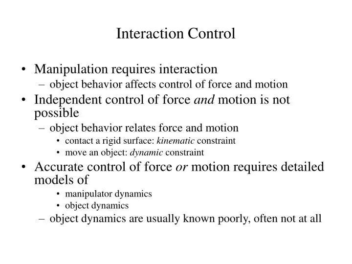
Interaction Control. Manipulation requires interaction object behavior affects control of force and motion Independent control of force and motion is not possible object behavior relates force and motion contact a rigid surface: kinematic constraint

E N D
Interaction Control • Manipulation requires interaction • object behavior affects control of force and motion • Independent control of force and motion is not possible • object behavior relates force and motion • contact a rigid surface: kinematic constraint • move an object: dynamic constraint • Accurate control of force or motion requires detailed models of • manipulator dynamics • object dynamics • object dynamics are usually known poorly, often not at all
Object Behavior • Can object forces be treated as external (exogenous) disturbances? • the usual assumptions don’t apply: • “disturbance” forces depend on manipulator state • forces often aren’t small by any reasonable measure • Can forces due to object behavior be treated as modeling uncertainties? • yes (to some extent) but the usual assumptions don’t apply: • command and disturbance frequencies overlap • Example: two people shaking hands • how each person moves influences the forces evoked • “disturbance” forces are state-dependent • each may exert comparable forces and move at comparable speeds • command & “disturbance” have comparable magnitude & frequency
Alternative: control port behavior • Port behavior: • system properties and/or behaviors “seen” at an interaction port • Interaction port: • characterized by conjugate variables that define power flow • Key point: port behavior is unaffected by contact and interaction
Impedance & Admittance • Impedance and admittance characterize interaction • a dynamic generalization of resistance and conductance • Usually introduced for linear systems but generalizes to nonlinear systems • state-determined representation: • this form may be derived from or depicted as a network model nonlinear 1D elastic element (spring)
Impedance & Admittance (continued) • Admittance is the causal dual of impedance • Admittance: flow out, effort in • Impedance: effort out, flow in • Linear system: admittance is the inverse of impedance • Nonlinear system: • causal dual is well-defined: • but may not correspond to any impedance • inverse may not exist
Impedance as dynamic stiffness • Impedance is also loosely defined as a dynamic generalization of stiffness • effort out, displacement in • Most useful for mechanical systems • displacement (or generalized position) plays a key role
Interaction control: causal considerations • What’s the best input/output form for the manipulator? • The set of objects likely to be manipulated includes • inertias • minimal model of most movable objects • kinematic constraints • simplest description of surface contact • Causal considerations: • inertias prefer admittance causality • constraints require admittance causality • compatible manipulator behavior should be an impedance • An ideal controller should make the manipulator behave as an impedance • Hence impedance control
Robot Impedance Control • Works well for interaction tasks: • Automotive assembly • (Case Western Reserve University, US) • Food packaging • (Technical University Delft, NL) • Hazardous material handling • (Oak Ridge National Labs, US) • Automated excavation • (University of Sydney, Australia) • … and many more • Facilitates multi-robot / multi-limb coordination: • Schneider et al., Stanford • Enables physical cooperation of robots and humans • Kosuge et al., Japan • Hogan et al., MIT
OSCAR assembly robot E.D.Fasse & J.F.Broenink, U. Twente, NL
Network modeling perspective on interaction control • Port concept • control interaction port behavior • port behavior is unaffected by contact and interaction • Causal analysis • impedance and admittance characterize interaction • object is likely an admittance • control manipulator impedance • Model structure • structure is important • power sources are commonly modeled as equivalent networks • Thévenin equivalent • Norton equivalent • Can equivalent network structure be applied to interaction control?
Equivalent networks • Initially applied to networks of static linear elements • Sources & linear resistors • Thévenin equivalent network • M. L. Thévenin, Sur un nouveau théorème d’électricité dynamique. Académie des Sciences, Comptes Rendus 1883, 97:159-161 • Thévenin equivalent source—power supply or transfer • Thévenin equivalent impedance—interaction • Connection—series / common current / 1-junction • Norton equivalent network is the causal dual form • Subsequently applied to networks of dynamic linear elements • Sources & (linear) resistors, capacitors, inductors
Nonlinear equivalent networks • Can equivalent networks be defined for nonlinear systems? • Nonlinear impedance and admittance can be defined as above • Thévenin & Norton sources can also be defined • Hogan, N. (1985) Impedance Control: An Approach to Manipulation. ASME J. Dynamic Systems Measurement & Control, Vol. 107, pp. 1-24. • However… • In general the junction structure cannot • In other words: • separating the pieces is always possible • re-assembling them by superposition is not
Nonlinear equivalent network for interaction control • One way to preserve the junction structure: • specify an equivalent network structure in the (desired) interaction behavior • provides key superpositionproperties • Specifically: • nodic desired impedance • does not require inertial reference frame • “virtual” trajectory • “virtual” as it need not be a realizable trajectory
Virtual trajectory • Nodic impedance • Defines desired interaction dynamics • Nodic because input velocity is defined relative to a “virtual” trajectory • Virtual trajectory: • like a motion controller’s reference or nominal trajectory but no assumption that dynamics are fast compared to nodic impedance object motion • “virtual” because it need not be realizable • e.g., need not be confined to manipulator’s workspace
Superposition of “impedance forces” • Minimal object model is an inertia • it responds to the sum of input forces • in network terms: it comes with an associated 1-junction • This guarantees linear summation of component impedances… • …even if the component impedances are nonlinear
One application: collision avoidance • Impedance control also enables non-contact (virtual) interaction • Impedance component to acquire target: • Attractive force field (potential “valley”) • Impedance component to prevent unwanted collision: • Repulsive force-fields (potential “hills”) • One per object (or part thereof) • Total impedance is the sum of these components • Simultaneously acquires target while preventing collisions • Works for moving objects and targets • Update their location by feedback to the (nonlinear) controller • Computationally simple • Initial implementation used 8-bit Z80 processors • Andrews & Hogan, 1983 Andrews,J. R. and Hogan, N. (1983) Impedance Control as a Framework for Implementing Obstacle Avoidance in a Manipulator, pp. 243-251 in D. Hardt and W.J. Book, (eds.), Control of Manufacturing Processes and Robotic Systems, ASME.
High-speed collision avoidance • Static protective (repulsive) fields must extend beyond object boundaries • may slow the robot unnecessarily • may occlude physically feasible paths • especially problematical if robot links are protected • Solution: time-varying impedance components • protective (repulsive) fields grow as robot speeds up, shrink as it slows down • Fields shaped to yield maximum acceleration or deceleration • Newman & Hogan, 1987 • See also extensive work by Khatib et al., Stanford Newman,W. S. and Hogan, N. (1987) High Speed Robot Control and Obstacle Avoidance Using Dynamic Potential Functions, proc. IEEE Int. Conf. Robotics & Automation, Vol. 1, pp. 14-24.
Impedance Control Implementation • Controlling robot impedance is an ideal • like most control system goals it may be difficult to attain • How do you control impedance or admittance? • One primitive but highly successful approach: • Design low-impedance hardware • Low-friction mechanism • Kinematic chain of rigid links • Torque-controlled actuators • e.g., permanent-magnet DC motors • high-bandwidth current-controlled amplifiers • Use feedback to increase output impedance • (Nonlinear) position and velocity feedback control • “Simple” impedance control
Robot Model • Robot Model θ: generalized coordinates, joint angles, configuration variables ω: generalized velocities, joint angular velocities τ: generalized forces, joint torques’ I: configuration-dependent inertia C: inertial coupling (Coriolis & centrifugal accelerations) G: potential forces (gravitational torques) • Linkage kinematics transform interaction forces to interaction torques X: interaction port (end-point) position V: interaction port (end-point) velocity Finteraction: interaction port force L: mechanism kinematic equations J: mechanism Jacobian
Simple Impedance Control • Target end-point behavior • Norton equivalent network with elastic and viscous impedance, possibly nonlinear • Express as equivalent (joint-space) configuration-space behavior • use kinematic transformations • This defines a position-and-velocity-feedback controller… • A (non-linear) variant of PD (proportional+derivative) control • …that will implement the target behavior
Mechanism singularities • Impedance control also facilitates interaction with the robot’s own mechanics • Compare with motion control: • Position control maps desired end-point trajectory onto configuration space (joint space) • Requires inverse kinematic equations • Ill-defined, no general algebraic solution exists • one end-point position usually corresponds to many configurations • some end-point positions may not be reachable • Resolved-rate motion control uses inverse Jacobian • Locally linear approach, will find a solution if one exists • At some configurations Jacobian becomes singular • Motion is not possible in one or more directions • A typical motion controller won’t work at or near these singular configurations
Mechanism junction structure • Mechanism kinematics relate configuration space {θ} to workspace {X} • In network terms this defines a multiport modulated transformer • Hence power conjugate variables are well-defined in opposite directions • Generalized coordinates uniquely define mechanism configuration • By definition • Hence the following maps are always well-defined • generalized coordinates (configuration space) to end-point coordinates (workspace) • generalized velocities to workspace velocity • workspace force to generalized force • workspace momentum to generalized momentum
Control at mechanism singularities • Simple impedance control law was derived by transforming desired behavior… • Norton equivalent network in workspace coordinates …from workspace to configuration (joint) space • All of the required transformations are guaranteed well-defined at all configurations • Hence the simple impedance controller can operate near, at and through mechanism singularities
Generalized coordinates • Aside: • Identification of generalized coordinates requires care • Independently variable • Uniquely define mechanism configuration • Not themselves unique • Actuator coordinates are often suitable, but not always • Example: Stewart platform • Identification of generalized forces also requires care • Power conjugates to generalized velocities • Actuator forces are often suitable, not always
Inverse kinematics • Generally a tough computational problem • Modeling & simulation afford simple, effective solutions • Assume a simple impedance controller • Apply it to a simulated mechanism with simplified dynamics • Guaranteed convergence properties • Hogan 1984 • Slotine &Yoerger 1987 • Same approach works for redundant mechanisms • Redundant: more generalized coordinates than workspace coordinates • Inverse kinematics is fundamentally “ill-posed” • Rate control based on Moore-Penrose pseudo-inverse suffers “drift” • Proper analysis of effective stiffness eliminates drift • Mussa-Ivaldi & Hogan 1991 Hogan, N. (1984) Some Computational Problems Simplified by Impedance Control, proc. ASME Conf. on Computers in Engineering, pp. 203-209. Slotine, J.-J.E., Yoerger, D.R. (1987) A Rule-Based Inverse Kinematics Algorithm for Redundant Manipulators Int. J. Robotics & Automation 2(2):86-89 Mussa-Ivaldi, F. A. and Hogan, N. (1991) Integrable Solutions of Kinematic Redundancy via Impedance Control. Int. J. Robotics Research, 10(5):481-491
Intrinsically variable impedance • Feedback control of impedance suffers inevitable imperfections • “parasitic” sensor & actuator dynamics • communication & computation delays • Alternative: control impedance using intrinsic properties of the actuators and/or mechanism • Stiffness • Damping • Inertia
Intrinsically variable stiffness • Engineering approaches • Moving-core solenoid • Separately-excited DC machine • Fasse et al. 1994 • Variable-pressure air cylinder • Pneumatic tension actuator • McKibben “muscle” • …and many more • Mammalian muscle • antagonist co-contraction increases stiffness & damping • complex underlying physics • see 2.183 • increased stiffness requires increased force Fasse, E. D., Hogan, N., Gomez, S. R., and Mehta, N. R. (1994) A Novel Variable Mechanical-Impedance Electromechanical Actuator. Proc. Symp. Haptic Interfaces for Virtual Environment and Teleoperator Systems, ASME DSC-Vol. 55-1, pp. 311-318.
Opposing actuators at a joint • Assume • constant moment arms • linear force-length relation • (grossly) simplified model of antagonist muscles about a joint f: force; l: length; k: actuator stiffness q: joint angle; t: torque; K: joint stiffness subscripts: g: agonist; n: antagonist, o: virtual • Equivalent behavior: • Opposing torques subtract • Opposing impedances add • Joint stiffness positive if actuator stiffness positive
Configuration-dependent moment arms • Connection of linear actuators usually makes moment arm vary with configuration • Joint stiffness, K: • Second term always positive • First term may be negative
This is the “tent-pole” effect • Consequences of configuration-dependent moment arms: • Opposing “ideal” (zero-impedance) tension actuators • agonist moment grows with angle, antagonist moment declines • always unstable • Constant-stiffness actuators • stable only for limited tension • Mammalian muscle: • stiffness is proportional to tension • good approximation of complex behavior • can be stable for all tension • Take-home messages: • Kinematics matters • “Kinematic” stiffness may dominate • Impedance matters • Zero output impedance may behighly undesirable
Intrinsically variable inertia • Inertia is difficult to modulate via feedback but mechanism inertia is a strong function of configuration • Use excess degrees of freedom to modulate inertia • e.g., compare contact with the fist or the fingertips • Consider the apparent (translational) inertia at the tip of a 3-link open-chain planar mechanism • Use mechanism transformation properties • Translational inertia is usually characterized by • Generalized (configuration space) inertia is • Jacobian: • Corresponding tip (workspace) inertia: • Snag: J(θ) is not square—inverse J(θ)-1 does not exist
Causal analysis • Inertia is an admittance • prefers integral causality • Transform inverse configuration-space inertia • Corresponding tip (workspace) inertia • This transformation is always well-defined • Does I(θ)-1always exist? • consider how we constructed I(θ) from individual link inertias • I(θ) must be symmetric positive definite, hence its inverse exists • Does Mtip-1 always exist? • yes, but sometimes it loses rank • inverse mass goes to zero in some directions—can’t move that way • causal argument: input force can always be applied • mechanism will “figure out” whether & how to move
Intrinsically variable damping • ER & MR fluids?
Other examples of “kinematic” stiffness • Stretched inelastic string • Check wave equation: • Bead in the middle of an inelastic wire • Relate to pulling a car from a ditch