Download
1 / 18
200 likes | 383 Vues
Atmospheric Boundary Layer Observations. Radio occultation bending angle and refractivity captures sharp inversions. RO bending angle captures altitude of sharp inversion. Radiosonde. Note: impact height ≈ height above surface + 2 km. Measured and reconstructed refractivity profiles.

E N D
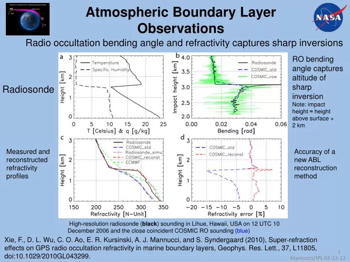
Atmospheric Boundary Layer Observations Radio occultation bending angle and refractivity captures sharp inversions RO bending angle captures altitude of sharp inversion Radiosonde Note: impact height ≈ height above surface + 2 km Measured and reconstructed refractivity profiles Accuracy of a new ABL reconstruction method High‐resolution radiosonde(black) sounding in Lihue, Hawaii, USA on 12 UTC 10 December 2006 and the close coincident COSMIC RO sounding (blue) Xie, F., D. L. Wu, C. O. Ao, E. R. Kursinski, A. J. Mannucci, and S. Syndergaard (2010), Super‐refraction effects on GPS radio occultation refractivity in marine boundary layers, Geophys. Res. Lett., 37, L11805, doi:10.1029/2010GL043299. Mannucci/JPL 02-13-12
Atmospheric Boundary Layer Height Eastern Pacific Stratocumulus Region Mean height VOCALS campaign region Height variability (std) Altitude maps (km) of the strong temperature inversion and sharp moisture gradient across the ABL top. RO shows significant ABL deepening in the western edge that is not captured in high-resolution ECMWF analyses (TL799L91). Period: Sept-Nov 2007-2009. F. Xie, D. L. Wu, C. O. Ao, A. J. Mannucci, and E. R. Kursinski (2012) “Advances and limitations of atmospheric boundary layer observations with GPS occultation over southeast Pacific Ocean” Atmos. Chem. Phys., 12, 903–918, 2012 doi:10.5194/acp-12-903-2012. Mannucci/JPL 02-13-12
Atmospheric Boundary Layer Height Global & Regional Climatology • Using RO to understand PBL height variations in different global regions. • Gradient methods work well for dry convective boundary layers that develop over subtropical deserts during daytime (e.g. Sahara). 2006-2009 Monthly averages of ABL heights in the Sahara region ERA – ECMWF-Interim reanalysis REF – refractivity criterion for height PWV – water vapor criterion for height Diurnal variation of ABL heights in the Sahara region, summer season JJA. Chi O. Ao, Duane E. Waliser, Steven K. Chan, Jui-Lin Li, BaijunTian, FeiqinXie, Anthony J. Mannucci (2012) Planetary Boundary Layer Heights from GPS Radio Occultation Refractivity and Humidity Profiles, submitted to JGR. Mannucci/JPL 02-13-12
New Algorithm to Retrieve Atmospheric Boundary Layer Moisture Varying moisture lapse • Strong inversion layers create ill-posed retrievals • New algorithm recovers set of possible retrievals based on Xie et al., 2006. • Adding GOES cloud top temperature breaks degeneracy • Recovered humidity profile detects presence of decoupled layer • Effective within or beneath heavy cloud cover • Uses GPS and GOES cloud top temperature Reference: Xie, F., S. Syndergaard, E. R. Kursinski, and B. M. Herman, 2006. An approach for retrieving marine boundary layer refractivity from GPS occultation data in the presence of superrefraction, J. Atmos. Ocean. Technol. 23(12), pp 1629–1644. Mannucci/JPL 02-13-12
Madden-Julian Oscillation Temperature Anomalies GPS AIRS Pressure (hPa) Composites of MJO temperature anomalies, tropics (10S-10N) 1 January 2006 to 31 December 2010 High resolution GPS data shows similar structures to AIRS but quantitative differences BaijunTian, Chi O. Ao, Duane E. Waliser, Eric J. Fetzer, Anthony J. Mannucci, and Joao Teixeira “Intraseasonal Temperature Variability in the Upper Troposphere and Lower Stratosphere from the GPS RO and AIRS Measurements”, in preparation (submission within 1-2 weeks) Mannucci/JPL 02-13-12
Comparisons Between RO and CMIP5 Model Runs • Assessing the CMIP5 model runs against 11 years of RO data • Using new Level-3 gridded RO products – monthly time series • 200 mb pressure surface geopotential height (~average layer temperature) Anomalies GPS shows better agreement in anomalies with atmosphere model, less agreement with coupled models Larger biases referenced to GPS in coupled models (ocean-atm CNRM, BCC), than in atmosphere-only model (uncoupled, CCCMA) C. O. Ao, A. J. Mannucci, J. Jiang, C. Zhai, H. Su, J. Cole, L. Donner, M. Ringer, A. Del Genio (2012) “Geopotentialheight field comparison between CMIP5 simulations and GPS radio occultation measurements,” to be submitted by July 31, 2012 deadline for consideration in AR5. Mannucci/JPL 02-13-12
Diurnal Tide From RO Diurnal variations in the stratosphere Amplitudes of the diurnal temperature tide at 9 hPa (~32 km) as a function of latitude (30S–30 N) and month of COSMIC RO observations from 2007 to 2009. The contour interval is 0.25 K. Gray shading indicates acceptable signal to noise ratio in recovering amplitude of diurnal tide. F. Xie, D. L. Wu, C. O. Ao, and A. J. Mannucci (2010) “Atmospheric diurnal variations observed with GPS radio occultation soundings”, Atmos. Chem. Phys., 10, 6889–6899, 2010, doi: 10.5194/acp-10-6889-2010 Mannucci/JPL 02-13-12
Stratospheric Drying Events “Cold events” have a significant impact on large-scale drying of the stratosphere Tropopause/Lower Stratosphere COSMIC Temperature Aura Water Vapor Takashima, H., N. Eguchi, and W. Read (2010), A short‐duration cooling event around the tropical tropopause and its effect on water vapor, Geophys. Res. Lett., 37, L20804, doi:10.1029/2010GL044505. Mannucci/JPL 02-13-12
Thin Cirrus Case Study Thin cirrus clouds in the Tropical TropopauseLayer (TTL) and their important ramifications for radiativetransfer, stratospheric humidity, and vertical transport CALPISO thin cirrus observations COSMIC RO temperatures J. R. Taylor, W. J. Randel, and E. J. Jensen, Cirrus cloud-temperature interactions in the tropical tropopauselayer: a case study Atmos. Chem. Phys., 11, 10085–10095, 2011, doi:10.5194/acp-11-10085-2011 Mannucci/JPL 02-13-12
Global Tropopause Structure Global tropopause climatology from COSMIC, and comparisons to NCEP-NCAR Reanalysis (NNR) “Although the NNR tropopause data have been widely used in climate studies, they are found to have significant and systematic biases, especially in the subtropics. This suggests that the NNR tropopause data should be treated with great caution in any quantitative studies.” From Son et al., 2011. Son, S.‐W., N. F. Tandon, and L. M. Polvani (2011), The fine‐scale structure of the global tropopause derived from COSMIC GPS radio occultation measurements, J. Geophys. Res., 116, D20113, doi:10.1029/2011JD016030. Mannucci/JPL 02-13-12
Static Stability of the Atmosphere Measure the long-term mean structure and variability of the global static stability field in the stratosphere and upper troposphere. S-2 Annual-mean, zonal-mean static stability (N2) in (top) conventional vertical coordinates and (bottom) tropopause-relative vertical coordinates. CHAMP RO data from 2002-2008. “The GPS temperature dataset offers the only global, high vertical resolution measurements of atmospheric temperature: select radiosondes have comparable vertical resolution but cover only a fraction of the globe; other satellite temperature products provide global coverage but have coarse vertical resolution.” Grise et al., 2010 Kevin M. Grise, David W. J. Thompson, And Thomas Birner (2010) A Global Survey of Static Stability in the Stratosphere and Upper Troposphere, J Clim 23, p. 2275, DOI:10.1175/2009JCLI3369.1 Mannucci/JPL 02-13-12
Air Pollution and Static Stability Understanding vertical mixing of commercial aviation emissions from cruise altitude to the surface Jet fuel burned by commercial aircraft in the year 2006 as a function of latitude (degrees) and TR altitude (km). The fuel burn is zonally and annually summed. The dark lines are contours of static stability derived from CHAMP and COSMIC data, zonally and annually averaged. Whitt, D. B., M. Z. Jacobson, J. T. Wilkerson, A. D. Naiman, and S. K. Lele (2011), Vertical mixing of commercial aviation emissions from cruise altitude to the surface, J. Geophys. Res., 116, D14109, doi:10.1029/2010JD015532. Mannucci/JPL 02-13-12
Southern Polar Precipitation Trends Assessment of Precipitation Changes over Antarctica and the Southern Ocean since 1989 in Contemporary Global Reanalyses Precipitation Net Precipitation Assimilation of COSMIC data into the ERA-Int and CFSR reanalyses begins in 2006. These diverge from the other reanalyses at that time. David H. Bromwich And Julien P. Nicolas, Andrew J. Monaghan (2011), An Assessment of Precipitation Changes over Antarctica and the Southern Ocean since 1989 in Contemporary Global Reanalyses, J. Clim 24, p. 4189, DOI10.1175/2011JCLI4074.1 . Mannucci/JPL 02-13-12
Longwave Forcing and Feedback RO helps determine these feedbacks Derived from Huang et al., Table 2 “We have demonstrated that when the two measurements are jointly used to quantify the feedbacks, the additional information provided by the GNSS RO measurement can be critically helpful to improve the accuracy in the results.” Yi Huang, Stephen S. Leroy, And James G. Anderson (2010) Determining Longwave Forcing and Feedback Using Infrared Spectra and GNSS Radio Occultation, J Clim 23, p. 6027, DOI: 10.1175/2010JCLI3588.1 Mannucci/JPL 02-13-12
Operational Impact Ron Gelaro, NASA/GMAO From Ector et al. presentation AMS Annual Meeting, January 2012 Mannucci/JPL 02-13-12
Operational Impact Relative FC error reduction per system The forecast sensitivity (Cardinali, 2009, QJRMS, 135, 239-250) denotes the sensitivity of a forecast error metric (dry energy norm at 24 or 48-hour range) to the observations. The forecast sensitivity is determined by the sensitivity of the forecast error to the initial state, the innovation vector, and the Kalman gain. (C. Cardinali) Relative FC error reduction per observation Use of Satellite Data at ECMWF P. Bauer Ⓒ ECMWF Mannucci/JPL 02-13-12
Hurricane Forecasting Impact (1) The impact of using RO refractivity observations on analyses and forecasts of Hurricane Ernesto’s genesis (2006) Observed Conventional data assimilated All available RO data + CTRL data RO data only above 6 km + CTRL data Ensemble mean of 48-h forecasts of Ernesto’s central sea level pressure (hPa) initialized from the analyses at 0000 UTC 25 Aug 2006. Note: CTRL uses radiosonde temperature, winds, and specific humidity, aircraft winds and temperature, satellite cloud drift winds, and surface station pressure observations. Satellite infrared and microwave sounders, radiances, and images are not assimilated. Hui Liu, Jeffrey Anderson, And Ying-hwaKuo (2012) Improved Analyses and Forecasts of Hurricane Ernesto’s Genesis Using Radio Occultation Data in an Ensemble Filter Assimilation System, Monthly Weather Review, v140, p. 151 DOI: 10.1175/MWR-D-11-00024.1 Mannucci/JPL 02-13-12
Hurricane Forecasting Impact (2) The ensemble mean of the total column cloud liquid water of the 48-h forecasts initialized from the RO, RO above 6-km, and CTRL analyses at 0000 UTC 25 Aug 2006. Units: log(kg kg-1). The observations of the actual storm are from satellite IR cloud images. Hui Liu, et al. (2012) Monthly Weather Review, v140, p. 151 DOI: 10.1175/MWR-D-11-00024.1 Mannucci/JPL 02-13-12