Download

1 / 39
390 likes | 568 Vues
LEARNING OBJECTIVES. Calculating two-asset portfolio expected returns and standard deviations Estimating measures of the extent of interaction – covariance and correlation coefficients

E N D
LEARNING OBJECTIVES • Calculating two-asset portfolio expected returns and standard deviations • Estimating measures of the extent of interaction – covariance and correlation coefficients • Being able to describe dominance, identify efficient portfolios and then apply utility theory to obtain optimum portfolios • Recognise the properties of the multi-asset portfolio set and demonstrate the theory behind the capital market line
One year: Holding period returns Where: s = semi-annual rate R = annual rate For three year holding period
EXAMPLE: Initial share price = £1.00 Share price three years later = £1.20 Dividends: year 1 = 6p, year 2 = 7p, year 3 = 8p
EXPECTED RETURNS AND STANDARD DEVIATION FOR SHARES Ace plc A share costs 100p to purchase now and the estimates of returns for the next year are as follows: Event Estimated Estimated Retur n Pr obability selling price, P dividend, D R 1 1 i Economic boom 114p 6p +20% 0.2 Nor mal gr owth 100p 5p +5% 0.6 Recession 86p 4p –10% 0.2 1.0
n p i i = 1 p i Expected returns 5 or 5% THE EXPECTED RETURN R R = i where R = expected r etur n R = return if event i occurs i = pr obability of event i occur ring n = number of events Expected return, Ace plc Event Pr obability of Retur n event pi Ri Ri pi Boom 0.2 +20 4 Gr owth 0.6 +5 3 Recession 0.2 –10 –2
STANDARD DEVIATION n 2 p ( ) = R – R i i =1 i Standard deviation, Ace plc Deviation squared probability Probability Return Expected return Deviation pi – – pi Ri (Ri Ri Ri Ri Ri ) 2 0.2 20% 5% 15 45 0.6 5% 5% 0 0 0.2 –10% 5% –15 45 Variance 90 2 Standard deviation 9.49%
Returns for a share in Bravo plc Event Return Probability Ri pi Boom –15% 0.2 Growth +5% 0.6 Recession +25% 0.2 1.0 Expected return on Bravo (–15 0.2) + (5 0.6) + (25 0.2) = 5 per cent Standard deviation, Bravo plc Deviation squared probability Probability Return Expected return Deviation pi – – pi Ri (Ri Ri Ri Ri ) Ri 2 –20 0.2 –15% 5% 80 0 0.6 +5% 5% 0 +20 0.2 +25% 5% 80 1.0 160 Variance 2 Standard deviation 12.65%
+ Return % – + Return % 3 4 1 2 5 6 8 7 – COMBINATIONS OF INVESTMENTS Hypothetical pattern of return for Ace plc 20 5 3 4 1 2 5 6 8 7 Time (years) –10 Hypothetical pattern of returns for Bravo plc 25 5 0 Time (years) –15
+ Return % – Returns over one year from placing £571 in Ace and £429 in Bravo Event Returns Returns Overall returns Percentage Ace Bravo on £1,000 r eturns £ £ Boom 571(1.2) = 685 429 – 429(0.15) = 365 1,050 5% Growth 571(1.05) = 600 429(1.05) = 450 1,050 5% Recession 571 – 571(0.1) = 514 429 (1.25) = 536 1,050 5% Hypothetical pattern of returns for Ace, Bravo and the two-asset portfolio Bravo 25 20 Portfolio 5 0 3 4 1 2 5 6 8 7 Time (years) –10 Ace –15
PERFECT NEGATIVE CORRELATION PERFECT POSITIVE CORRELATION Annual returns on Ace and Clara Event Pr obability Retur ns Retur ns p on Ace on Clara i i % % Boom 0.2 +20 +50 Growth 0.6 +5 +15 Recession 0.2 –10 –20 Returns over a one-year period from placing £500 in Ace and £500 in Clara Event Returns Returns Overall Percentage i Ace Clara return on r eturn £ £ £1,000 Boom 600 750 1,350 35% Growth 525 575 1,100 10% Recession 450 400 850 –15%
Hypothetical patterns of returns for Ace and Clara 50 Clara Portfolio 20 + 5 Ace 1 2 3 4 5 6 7 8 T ime – (years) –10 –15 –20
Return Probability Return Probability – 25 0.5 = –12.5 –25 0.5 = –12.5 35 0.5 = 17.5 35 0.5 = 17.5 5.0% 5.0% INDEPENDENT INVESTMENTS Expected returns for shares in X and shares in Y Expected return for shares in X Expected return for shares in Y Standard deviations for X or Y as single investments Deviations squared probability Return Probability Expected return Deviations pi Ri – R Ri Ri (Ri – R)2 pi –25% 0.5 5% –30 450 35% 0.5 5% 30 450 Variance 900 Standard deviation 30%
Exhibit 7.17 A mixed portfolio: 50 per cent of the fund invested in X and 50 per cent in Y, expected return Possible Joint Joint Retur n outcome returns probability pr obability combinations Both firms do badly –25 0.5 0.5 = 0.25 –25 0.25 = –6.25 X does badly Y does well 5 0.5 0.5 = 0.25 5 0.25 = 1.25 X does well Y does badly 5 0.5 0.5 = 0.25 5 0.25 = 1.25 Both firms do well 35 0.5 0.5 = 0.25 35 0.25 = 8.75 Expected return 1.00 5.00% Standard deviation, mixed portfolio Deviations squared probability Return Probability Expected return Deviations pi (Ri – R)2 pi Ri R Ri – R –25 0.25 5 –30 225 5 0.50 5 0 0 35 0.25 5 30 225 Variance 450 Standard deviation 21.21%
A CORRELATION SCALE • So long as the returns of constituent assets of a portfolio are not perfectly positively correlated, diversification can reduce risk. The degree of risk reduction depends on: • the extent of statistical interdependence • between the returns of the different • investments: the more negative the better; and • the number of securities over which to spread • the risk: the greater the number, the lower the • risk. –1 0 +1 Perfect Independent Perfect negative positive correlation correlation Correlation scale
pi RA THE EFFECTS OF DIVERSIFICATION WHEN SECURITY RETURNS ARE NOT PERFECTLY CORRELATED Returns on shares A and B for alternative economic states Event i Pr obability Retur n on A Retur n on B State of the economy pi RA RB Boom 0.3 20% 3% Gr owth 0.4 10% 35% Recession 0.3 0% –5% Company A: Expected return Pr obability Return pi RA 0.3 20 6 0.4 10 4 0.3 0 0 10% Company A: Standard deviation Deviation squared probability Expected Probability Return r eturn Deviation RA pi RA (RA – RA) (RA – RA)2 pi 0.3 20 10 10 30 0.4 10 10 0 0 0.3 0 10 –10 30 60 Variance Standard deviation 7.75%
Company B: Expected return Probability Return RB pi pi RB 0.3 3 0.9 0.4 35 14.0 0.3 –5 –1.5 13.4% Company B: Standard deviation Deviation squared probability Expected Deviation Probability Return return pi (RB – RB)2 pi RB (RB – RB) RB 0.3 3 13.4 10.4 32.45 0.4 35 13.4 21.6 186.62 0.3 –5 13.4 –18.4 101.57 Variance 320.64 = 17.91% Standard deviation Summary table: Expected returns and standard deviations for Companies A and B Expected return Standard deviation Company A Company B 10% 13.4% 7.75% 17.91%
A general rule in portfolio theory: Portfolio returns are a weighted average of the expected returns on the individual investment… BUT… Portfolio standard deviation is less than the weighted average risk of the individual investments, except for perfectly positively correlated investments. Exhibit: 7.26 Return and standard deviation for shares in firms A and B 20 15 B P 10 A Expected return R % Q 5 5 10 15 20 Standard deviation %
PORTFOLIO EXPECTED RETURNS AND STANDARD DEVIATION • 90 per cent of the portfolio funds are placed in A • 10 per cent are placed in B Expected returns, two-asset portfolio • Proportion of funds in A = a = 0.90 • Proportion of funds in B = 1 – a = 0.10 Rp = aRA + (1 – a)RB Rp = 0.90 10 + 0.10 13.4 = 10.34% p = a22A + (1 – a)22B + 2a (1 – a) cov (RA, RB) wher e p = portfolio standard deviation A = variance of investment A B= variance of investment B cov (RA, RB) = covariance of A and B
n cov (RA, RB) = {(RA – RA)(RB – RB)pi} i = 1 COVARIANCE The covariance formula is: Exhibit 7.27 Covariance Event and Expected Deviation of A pr obability of Returns r etur ns Deviations deviation of B pr obability )pi event pi R R R R R – R R – R (R – R )(R – R A A B B B A B A B A A B Boom 0.3 20 3 10 13.4 10 –10.4 10 –10.4 0.3 = –31.2 Gr owth 0.4 10 35 10 13.4 0 21.6 0 21.6 0.4 = 0 Recession 0.3 0 –5 10 13.4 –10 –18.4 –10 –18.4 0.3 = 55.2 Covariance of A and B, cov ( R , R ) = +24 A B
Invested in a portfolio (90% in A, 10% in B) 20 Portfolio (A=90%, B=10%) 15 Expected return R % 10 5 20 15 10 5 Standard deviation % STANDARD DEVIATION p = a22A + (1 – a)22B + 2a (1 – a) cov (RA, RB) p = 0.902 60 + 0.102 320.64 + 2 0.90 0.10 24 p = 48.6 + 3.206 + 4.32 p = 7.49% Exhibit 7.28 Summary table: expected return and standard deviation Expected return (%) Standard deviation (%) All invested in Company A 10 7.75 All invested in Company B 13.4 17.91 10.34 7.49 Exhibit 7.29 Expected returns and standard deviation for A and B and a 90:10 portfolio of A and B B A
CORRELATION COEFFICIENT cov (RARB) RAB = RAB = = +0.1729 If RAB = then cov (RARB) = p = a22A + (1 – a)2 2B + 2a (1 – a) AB 24 7.75 17.91 cov (RARB) RABAB AB RABAB
Returns on G Returns on F Returns on G Returns on F Exhibit 7.30 Perfect positive correlation Returns on G Returns on F Exhibit 7.31 Perfect negative correlation Exhibit 7.32 Zero correlation coefficient
DOMINANCE AND THE EFFICIENT FRONTIER Exhibit 7.33 Returns on shares in Augustus and Brown Event (weather for season) Returns on Augustus Probability of event Returns on Brown pi RB RA Warm 20% –10% 0.2 Average 0.6 15% 22% 0.2 Wet 10% 44% Expected return 20% 15% Exhibit 7.34 Standard deviation for Augustus and Brown Probability Returns Returns pi on Augustus on Brown (RA – RA)2 pi (RB – RB)2 pi RA 0.2 20 5 –10 180.0 0.6 15 0 22 2.4 0.2 10 5 44 115.2 Variance, Variance, B 10 297.6 Standard deviation, B Standard deviation, 3.162 17.25
Exhibit 7.35 Covariance Deviation of A deviation of B probability Expected Deviations returns Probability Returns pi (RA –RA)(RB –RB)pi RA RB RA –RA RB –RB RA RB 0.2 20 –10 15 20 5 –30 5 –30 0.2 = –30 0.6 15 22 15 20 0 2 0 2 0.6 = 0 0.2 10 44 15 20 –5 24 –5 24 0.2 = –24 Covariance (RA RB) –54 cov (RA, RB) RAB = AB –54 RAB = = –0.99 3.162 17.25
return (%) Expected (%) Brown weighting weighting Augustus (%) =17.25 = 1.01 = 3.16 = 1.16 = 0.39 = 7.06 =12.2 Standard deviation 0.252 10 + 0.752 297.6 + 2 0.25 0.75 –54 0.852 10 + 0.152 297.6 + 2 0.85 0.15 –54 0.52 10 + 0.52 297.6 + 2 0.5 0.5 –54 0.82 10 + 0.22 297.6 + 2 0.8 0.2 –54 0.92 10 + 0.12 297.6 + 2 0.9 0.1 –54 Exhibit 7.36 Risk-return correlations: two-asset portfolios for Augustus and Brown 15.75 18.75 15 16.0 17.5 15.5 20 75 0 15 20 100 50 10 0 50 25 90 85 80 100 J B K M L N A Portfolio
Exhibit 7.37 Risk-return profile for alternative portfolios of Augustus and Brown 21 B 20 19 N 18 M Efficiency frontier Return Rp % 17 L 16 K J 15 A 3 5 6 18 1 2 4 7 8 9 10 11 12 13 14 15 16 17 p Standard deviation
If a fund is to be split between two securities, A and B, and a is the fraction to be allocated to A, then the value for a which results in the lowest standard deviation is given by: FINDING THE MINIMUM STANDARD DEVIATION FOR COMBINATIONS OF TWO SECURITIES
INDIFFERENCE CURVES Exhibit 7.38 Indifference curve for Mr Chisholm X 14 Z Indifference curve I 105 Return % 10 W Y 16 20 Standard deviation %
Exhibit 7.39 A map of indifference curves North-west I 129 I 121 I 110 I 107 S I 105 Return % T 14 Z 10 W South-west 16 20 Standard deviation %
Exhibit 7.40 Intersecting indifference curves I105 I101 M Return % I101 I105 Standard deviation %
Exhibit 7.41 Varying degrees of risk aversion as represented by indifference curves Return % Return % Return % Standard deviation % Standard deviation % Standard deviation % (a) Moderate risk aversion (b) Low risk aversion (c) High risk aversion
CHOOSING THE OPTIMAL PORTFOLIO Exhibit 7.42 Optimal combination of Augustus and Brown I 21 3 I 2 B 20 I 1 19 N Efficiency frontier Return % 18 M 17 L 16 K J 15 A 1 2 3 4 5 6 7 8 9 10 11 12 13 14 15 16 17 18 Standard deviation % p
THE BOUNDARIES OF DIVERSIFICATION Exhibit 7.44 The boundaries of diversification D 22 21 20 RCD = –1 19 RCD = +1 H 18 Return % RCD = 0 17 E G 16 F 15 C Return % 1 2 3 4 5 6 7 8 9 10 Standard deviation % p
EXTENSION TO A LARGE NUMBER OF SECURITIES Exhibit 7.47 A three-asset portfolio A 4 1 3 B Return 2 C Standard deviation
Exhibit 7.48 The opportunity set for multi-security portfolios and portfolio selection for a highly risk-averse person and for a slightly risk-averse person IL3 Efficiency frontier IL2 IL1 V IH3 IH2 IH1 U Return Inefficient region Inefficient region Standard deviation
THE CAPITAL MARKET LINE Exhibit 7.53 Combining risk-free and risky investments M F Return C B rf A Standard deviation
Exhibit 7.54 Indifference curves applied to combinations of the market portfolio and the risk-free asset M Return Y X rf Standard deviation
Exhibit 7.55 The capital market line Capital market line N T S M Return G H rf Standard deviation
Problems with portfolio theory: • relies on past data to predict future risk and • return • involves complicated calculations • indifference curve generation is difficult • few investment managers use computer • programs because of the nonsense results • they frequently produce