Download
1 / 25
250 likes | 361 Vues
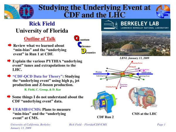
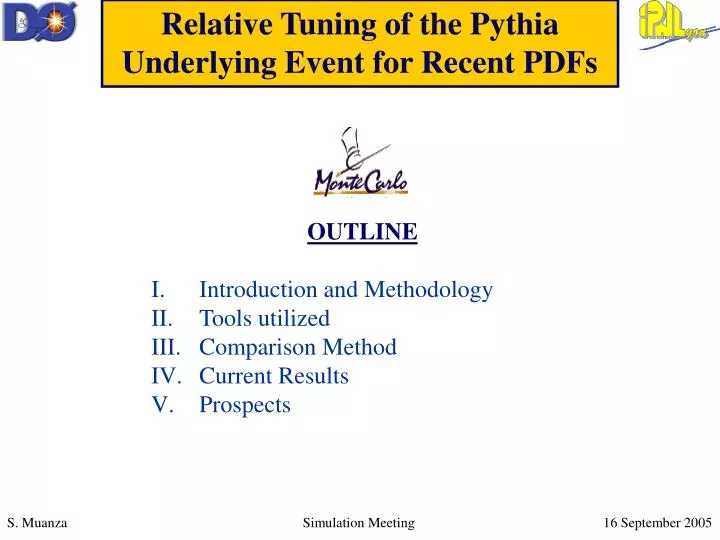
Relative Tuning of the Pythia Underlying Event for Recent PDFs. OUTLINE Introduction and Methodology Tools utilized Comparison Method Current Results Prospects. I. Introduction.

E N D
Relative Tuning of the Pythia Underlying Event for Recent PDFs • OUTLINE • Introduction and Methodology • Tools utilized • Comparison Method • Current Results • Prospects Simulation Meeting 16 September 2005
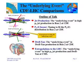
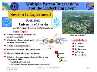
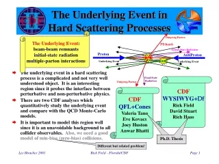
I. Introduction • A quite detailed study of the underlying event has been performed by Rick Field a theorist working in the CDF collaboration (http://www.phys.ufl.edu/~rfield/cdf/rdf_talks.html) • This study has been sustained for more than 5 years • Working definition of the Underlying Event: • All but the hard scattering process • ie: beam-beam remnants (spectator partons), plus possible ISR gluon radiations ,plus the possible Multiple Parton Interactions (MPI) • Systematic comparisons of CDF Run I data (min.bias and soft jets) to different MC models have been performed and finally led to a tuning of Pythia underlying event model: Simulation Meeting 16 September 2005
I. Introduction Simulation Meeting 16 September 2005
I. Introduction • This tuning is PDF dependent (http://cepa.fnal.gov/patriot/mc4run2/MCTuning/run2mc/R_Field.pdf) • This tuning fits CDF Run IIA min.bias+soft jets data • Provided decent choice for the renormalization scales, this tuning also fits the UE for the bbbar, di-photon, Z+jets processes (http://www.phys.ufl.edu/~rfield/cdf/RickField_Workshop_6-11-04.pdf) Simulation Meeting 16 September 2005
I. Methodolgy • Since the UE tuning is PDF dependentit should in principle be redone whenever changing from the “reference PDF” (CTEQ5L for Tune A) • However this is obviously cumbersome since it requires correcting either the data or the detailed MC and re-doing the full tuning procedure each time • I propose instead to start from a reference (CTEQ5L for Tune A) that was properly tuned to data and just to reproduce its UE properties • This only requires generator level or fast simulation scan over the UE parameters: whatever set of parameters that reproduces the reference UE constitutes the relative UE tuning for a given PDF • I assume the p/pbar hadronic matter is described by a double gaussian (MSTP(82)=4 as in Tune A), so I’m left w/ scanning “only” over 7 PARP parameters (67,82-86,90) since PARP(89)=1800.0 keeps its fixed value (all the evolutions to another CoM energy are internally treated within Pythia) Simulation Meeting 16 September 2005
I. Methodolgy Scan over the UE Parameters This scan contains 3888 different PARP configurations Simulation Meeting 16 September 2005
II. Tools Utilized • Generator: • Pythia v6.320 • PDF Library: • LHAPDF v4.0 • Fast detector simulation: • ATLFAST v2.60 (Atlas Collaboration), including smeared tracks and jets • Events production: • Process: • Pythia minbias MSEL=2 MSUB(91-95) • elastic scattering+ diffraction + low pT QCD, w/ pT* > 0 GeV • Note: the soft jets part is not yet produced ( MSEL=1, w/ pT* > 5 GeV) • Statistics: • 25k / sample (ie per PDF/ & per PARP combination) • PDF: • ref. sample: • CTEQ5L (LO fit & LO aS) • compar. sample: • CTEQ6LL, ALEKHIN02LO, MRST01LO (LO fit & LO aS) • CTEQ6L (LO fit & NLO aS) Simulation Meeting 16 September 2005
II. Tools Utilized • Events selection: • Similar to R. Field's: • events w/ 1 or 2 jets, pT(jets)> 0 GeV, |eta(jets)|<2.0 • The transverse plane is divided into 4 regions: • towards: |Df(ojbect,leading jet)|<60° • away: | Df(ojbect, leading jet)|>120° (only for 2 jet events) • transverse regions: 60°<|Df(ojbect,leading jet)|<120° • Look at tracks w/ pT(tracks)>0.5 GeV and |eta(tracks)|<1.0 in the transverse regions • Construct 2-D histos: • Ntracks/Dh/Df/(1 GeV)vs leading jet pT • SpT/ Dh/Df/(1 GeV)vs leading jet pT (scalar pT sum) • Differences wrt R. Field: • I used "calorimeter jets" instead of “track jets” • => pT(jets)>6 Gev instead of 0 GeV • Note: • the overall efficiency is rather low (~12%) and since I did not write any filter for the produced events, the comparisonsare only based on a KS test of two 2-D histos w/ ~3 k entries!!! Simulation Meeting 16 September 2005
Charged Particle DfCorrelations • Look at charged particle correlations in the azimuthal angle Df relative to the leading charged particle jet. • Define |Df| < 60o as “Toward”, 60o < |Df| < 120o as “Transverse”, and |Df| > 120o as “Away”. • All three regions have the same size in h-f space, DhxDf = 2x120o = 4p/3. Simulation Meeting 16 September 2005
Tuned PYTHIA 6.206 vs HERWIG 6.4“TransMAX/MIN” vs PT(chgjet#1) • Plots shows data on the “transMAX/MIN” <Nchg> and “transMAX/MIN” <PTsum> vs PT(chgjet#1). The solid (open) points are the Min-Bias (JET20) data. • The data are compared with the QCD Monte-Carlo predictions of HERWIG 6.4 (CTEQ5L, PT(hard) > 3 GeV/c) and two tuned versions of PYTHIA 6.206 (PT(hard) > 0, CTEQ5L, PARP(67)=1 and PARP(67)=4). <Nchg> <PTsum> Simulation Meeting 16 September 2005
III. Comparison Method • Histo Comparisons: for each PARP configuration and for each PDF, the two • 2-D histos are compared using a 2-D Kolmogorov-Smirnov test to those of the ref. sample (just the shapes enter the comparison, not the normalizations) • Global probability: the probability assigned to each comparison sample is simply the product [1] of the individual probability of comparing on one hand the charged tracks density and on the other hand the pTsum density • Tools: all the histos and comparison methods are taken from ROOT v4.04.02b Valid if & only if var1 and var2 are not correlated!!! Have to calculate a conditional probability if var1 and var2 are correlated!!! Simulation Meeting 16 September 2005
IV. Current Results • PDF: ALEKHIN02LO • LO fit and LO aS • 3881/3888 configs • Max(PKS)=0.967 008 (8 max configs) • Min(PKS)=2.058x10⁻¹⁰ (4 min configs) Simulation Meeting 16 September 2005
IV. Current Results • PDF: MRST01LO • LO fit and LO aS • 3820/3888 configs • Max(PKS)=0.956524 (12 max configs) • Min(PKS)=4.433x10⁻¹¹ (4 min configs) Simulation Meeting 16 September 2005
IV. Current Results • PDF: CTEQ6L • LO fit and NLO aS • 3867/3888 configs • Max(PKS)=0.954313 (12 max configs) • Min(PKS)=2.924x10⁻¹⁰ (4 min configs) Simulation Meeting 16 September 2005
IV. Current Results • PDF: CTEQ6LL • aka CTEQ6L1 • LO fit and LO aS • 3886/3888 configs • Max(PKS)=0.977060 (12 max configs) • Min(PKS)=1.815x10⁻¹¹ (4 min configs) Simulation Meeting 16 September 2005
IV. Current Results Example w/ Alekhin 2002 LO PDF ref best worst « same » HT (GeV) Simulation Meeting 16 September 2005
IV. Current Results ref best worst « same » mET (GeV) Simulation Meeting 16 September 2005
IV. Current Results ref best worst « same » N(jets) Simulation Meeting 16 September 2005
IV. Current Results ref best worst « same » Total N(tracks) Simulation Meeting 16 September 2005
IV. Current Results • After fixing the correlation issue: • Attaching file plots.root as _file0... • root [1] h2_hist1_mix0->GetCorrelationFactor(1,2) • (const Stat_t)1.22289661104907951e-01 • root [2] h2_hist1_mix1->GetCorrelationFactor(1,2) • (const Stat_t)8.79092032677424529e-01 • root [3] h2_hist2_mix0->GetCorrelationFactor(1,2) • (const Stat_t)1.18224432124161408e-01 • root [4] h2_hist2_mix1->GetCorrelationFactor(1,2) • (const Stat_t)8.23833825978842360e-01 • The correlation coefficient drops from 80% downto 12% • This makes the marginal probabilities product an acceptable approximation Var2=Ntracks/Dh/Df/(1 GeV) Var1=SpT/ Dh/Df/(1 GeV) Var1=(SpT/Ntracks)/ Dh/Df/(1 GeV) Simulation Meeting 16 September 2005
VI. Conclusions & Prospects • Conclusions: • There are flat directions (as expected in multivariate analyses, especially w/ coarse scans and limited statistics). In this case I propose to pick the PARP value which is the closest to the reference one (CTEQ5L+Tune A) • As expected the shape of the so-called “best” configuration (green histos) is the closest to that of the reference (black histos). This demonstate that there is a measurable difference between different UE settings for a given PDF and that the UE is PDF-dependent. • Prospects: • Produce the low pT QCD samples • Add them to the 2-D histos for the comparisons • Couple of additional cross checks • Increase the statistics Simulation Meeting 16 September 2005
VI. Prospects • Produce the low pT QCD samples • Add them to the 2-D histos for the comparisons • Couple of additional cross checks • Increase the statistics Simulation Meeting 16 September 2005
Back Up Simulation Meeting 16 September 2005
Pythia UE Parameters Definition Simulation Meeting 16 September 2005
VI. Final Checks on Shapes Simulation Meeting 16 September 2005