Download
1 / 40
410 likes | 617 Vues
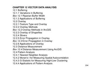
CHAPTER 12 VECTOR DATA ANALYSIS 12.1 Buffering 12.1.1 Variations in Buffering Box 12.1 Riparian Buffer Width 12.1.2 Applications of Buffering 12.2 Overlay 12.2.1 Feature Type and Overlay 12.2.2 Overlay Methods Box 12.2 Overlay Methods in ArcGIS 12.2.3 Overlay of Shapefiles

E N D
CHAPTER 12 VECTOR DATA ANALYSIS 12.1 Buffering 12.1.1 Variations in Buffering Box 12.1 Riparian Buffer Width 12.1.2 Applications of Buffering 12.2 Overlay 12.2.1 Feature Type and Overlay 12.2.2 Overlay Methods Box 12.2 Overlay Methods in ArcGIS 12.2.3 Overlay of Shapefiles 12.2.4 Slivers 12.2.5 Error Propagation in Overlay Box 12.3 Error Propagation in Overlay 12.2.6 Applications of Overlay 12.3 Distance Measurement Box 12.4 Distance Measurement Using ArcGIS 12.4 Pattern Analysis 12.4.1 Nearest Neighbor Analysis 12.4.2 Moran’s I for Measuring Spatial Autocorrelation 12.4.3 G-Statistic for Measuring High/Low Clustering 12.4.4 Applications of Pattern Analysis
12.5 Map Manipulation Box 12.5 Map Manipulation Using ArcGIS Key Concepts and Terms Review Questions Applications: Vector Data Analysis Task 1: Perform Buffering and Overlay Task 2: Overlay Multicomponent Polygons Task 3: Measure Distances Between Points and Lines Task 4: Compute General and Local G-statistics Challenge Question References
Vector Data Analysis • Vector data analysis uses the geometric objects of point, line, and polygon. • The accuracy of analysis results depends on the accuracy of these objects in terms of location and shape. • Topology can also be a factor for some vector data analyses such as buffering and overlay.
Buffering • Based on the concept of proximity, buffering creates two areas: one area that is within a specified distance of select features and the other area that is beyond. • The area that is within the specified distance is called the buffer zone. • There are several variations in buffering. The buffer distance can vary according to the values of a given field. Buffering around line features can be on either the left side or the right side of the line feature. Boundaries of buffer zones may remain intact so that each buffer zone is a separate polygon.
Figure 12.1 Buffering around points, lines, and areas.
Figure 12.2 Buffering with different buffer distances.
Figure 12.3 Buffering with four rings.
Figure 12.4 Buffer zones not dissolved (top) or dissolved (bottom).
Overlay • An overlayoperationcombines the geometries and attributes of two feature layers to create the output. • The geometry of the output represents the geometric intersection of features from the input layers. • Each feature on the output contains a combination of attributes from the input layers, and this combination differs from its neighbors.
Figure 12.5 Overlay combines the geometry and attribute data from two layers into a single layer. The dashed lines are not included in the output.
Feature Type and Overlay Overlay operations can be classified by feature type into point-in-polygon, line-in-polygon, and polygon-on-polygon.
Figure 12.6 Point-in-polygon overlay. The input is a point layer (the dashed lines are for illustration only and are not part of the point layer). The output is also a point layer but has attribute data from the polygon layer.
Figure 12.7 Line-in-polygon overlay. The input is a line layer (the dashed lines are for illustration only and are not part of the line layer). The output is also a line layer. But the output differs from the input in two aspects: the line is broken into two segments, and the line segments have attribute data from the polygon layer.
Figure 12.8 Polygon-on-polygon overlay. In the illustration, the two layers for overlay have the same area extent. The output combines the geometry and attribute data from the two layers into a single polygon layer.
Overlay Methods • All overlay methods are based on the Boolean connectors of AND, OR, and XOR. • An overlay operation is called Intersect if it uses the AND connector. • An overlay operation is called Union if it uses the OR connector. • An overlay operation that uses the XOR connector is called Symmetrical Difference or Difference. • An overlay operation is called Identity or Minus if it uses the following expression: [(input layer) AND (identity layer)] OR (input layer).
Figure 12.9 The Union method keeps all areas of the two input layers in the output.
Figure 12.10 The Intersect method preserves only the area common to the two input layers in the output. (The dashed lines are for illustration only; they are not part of the output.)
Figure 12.11 The Symmetric Difference method preserves only the area common to only one of the input layers in the output. (The dashed lines are for illustration only; they are not part of the output.)
Figure 12.12 The Identity method produces an output that has the same extent as the input layer. But the output includes the geometry and attribute data from the identity layer.
Slivers • A common error from overlaying polygon layers is slivers, very small polygons along correlated or shared boundary lines of the input layers. • To remove slivers, ArcGIS uses the cluster tolerance, whichforces points and lines to be snapped together if they fall within the specified distance.
Figure 12.13 The top boundary has a series of slivers. These slivers are formed between the coastlines from the input layers in overlay.
Figure 12.14 A cluster tolerance can remove many slivers along the top boundary (A) but can also snap lines that are not slivers (B).
Areal Interpolation One common application of overlay is to help solve the areal interpolation problem. Areal interpolationinvolves transferring known data from one set of polygons (source polygons) to another (target polygons).
Figure 12.15 An example of areal interpolation. Thick lines represent census tracts and thin lines school districts. Census tract A has a known population of 4000 and B has 2000. The overlay result shows that the areal proportion of census tract A in school district 1 is 1/8 and the areal proportion of census tract B, 1/2. Therefore, the population in school district 1 can be estimated to be 1500, or [(4000 x 1/8) + (2000 x 1/2)].
Pattern Analysis • Pattern analysis refers to the use of quantitative methods for describing and analyzing the distribution pattern of spatial features. • At the general level, a pattern analysis can reveal if a distribution pattern is random, dispersed, or clustered. • At the local level, a pattern analysis can detect if a distribution pattern contains local clusters of high or low values. • Pattern analysis includes nearest neighbor analysis, Moran’s I for measuring spatial autocorrelation, and G-statistic for measuring high/low clustering.
Figure 12.16 A point pattern showing deer locations.
Figure 12.17 A point pattern showing deer locations and the number of sightings at each location.
Figure 12.18 Percent Latino population by block group in Ada County, Idaho. Boise is located in the upper center of the map with small sized block groups.
Figure 12.19 Z scores for the Local Indicators of Spatial Association (LISA) by block group in Ada County, Idaho.
Figure 12.20 Z scores for the local G-statistics by block group in Ada County, Idaho.
Map Manipulation • Tools are available in a GIS package for manipulating and managing maps in a database. • These tools include Dissolve, Clip, Append, Select, Eliminate, Update, Erase, and Split.
Figure 12.21 Dissolve removes boundaries of polygons that have the same attribute value in (a) and creates a simplified layer (b).
Figure 12.22 Clip creates an output that contains only those features of the input layer that fall within the area extent of the clip layer. (The dashed lines are for illustration only; they are not part of the clip layer.)
Figure 12.23 Append pieces together two adjacent layers into a single layer but does not remove the shared boundary between the layers.
Figure 12.24 Select creates a new layer (b) with selected features from the input layer (a).
Figure 12.25 Eliminate removes some small slivers along the top boundary (A).
Figure 12.26 Update replaces the input layer with the update layer and its features. (The dashed lines are for illustration only; they are not part of the update layer.)
Figure 12.27 Erase removes features from the input layer that fall within the area extent of the erase layer. (The dashed lines are for illustration only; they are not part of the erase layer.)
Figure 12.28 Split uses the geometry of the split layer to divide the input layer into four separate layers.
CrimeStat http://www.icpsr.umich.edu/NACJD/crimestat.htm