Some Preliminary Results of GCEP

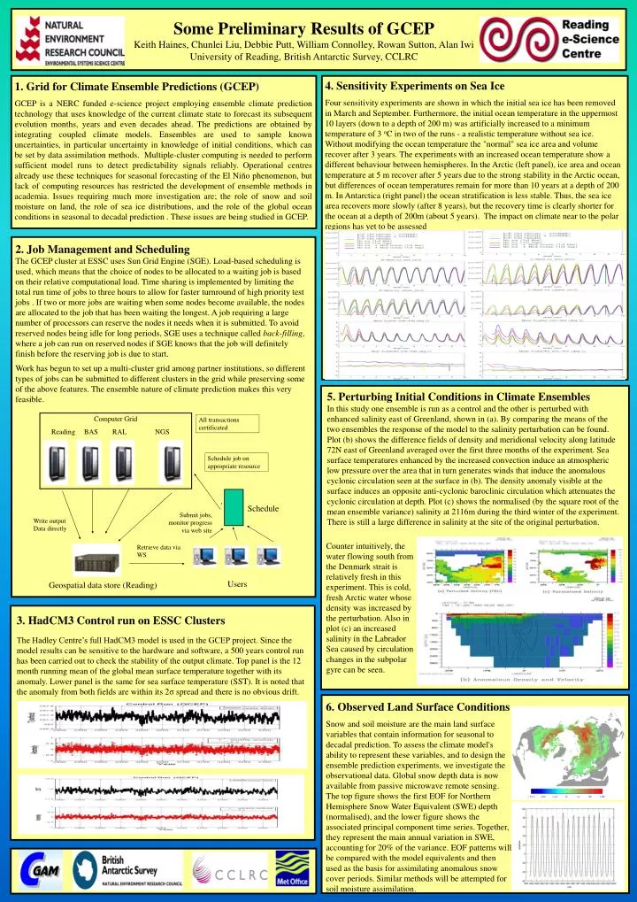
1. Some Preliminary Results of GCEP Keith Haines, Chunlei Liu, Debbie Putt, William Connolley, Rowan Sutton, Alan Iwi University of Reading, British Antarctic Survey, CCLRC 4. Sensitivity Experiments on Sea Ice Four sensitivity experiments are shown in which the initial sea ice has been removed in March and September. Furthermore, the initial ocean temperature in the uppermost 10 layers (down to a depth of 200 m) was artificially increased to a minimum temperature of 3 oC in two of the runs - a realistic temperature without sea ice.Without modifying the ocean temperature the "normal" sea ice area and volume recover after 3 years. The experiments with an increased ocean temperature show a different behaviour between hemispheres. In the Arctic (left panel), ice area and ocean temperature at 5 m recover after 5 years due to the strong stability in the Arctic ocean, but differences of ocean temperatures remain for more than 10 years at a depth of 200 m. In Antarctica (right panel) the ocean stratification is less stable. Thus, the sea ice area recovers more slowly (after 8 years), but the recovery time is clearly shorter for the ocean at a depth of 200m (about 5 years).  The impact on climate near to the polar regions has yet to be assessed 1. Grid for Climate Ensemble Predictions (GCEP) GCEP is a NERC funded e-science project employing ensemble climate prediction technology that uses knowledge of the current climate state to forecast its subsequent evolution months, years and even decades ahead. The predictions are obtained by integrating coupled climate models. Ensembles are used to sample known uncertainties, in particular uncertainty in knowledge of initial conditions, which can be set by data assimilation methods. Multiple-cluster computing is needed to perform sufficient model runs to detect predictability signals reliably. Operational centres already use these techniques for seasonal forecasting of the El Niño phenomenon, but lack of computing resources has restricted the development of ensemble methods in academia. Issues requiring much more investigation are; the role of snow and soil moisture on land, the role of sea ice distributions, and the role of the global ocean conditions in seasonal to decadal prediction . These issues are being studied in GCEP. 2. Job Management and Scheduling The GCEP cluster at ESSC uses Sun Grid Engine (SGE). Load-based scheduling is used, which means that the choice of nodes to be allocated to a waiting job is based on their relative computational load. Time sharing is implemented by limiting the total run time of jobs to three hours to allow for faster turnround of high priority test jobs . If two or more jobs are waiting when some nodes become available, the nodes are allocated to the job that has been waiting the longest. A job requiring a large number of processors can reserve the nodes it needs when it is submitted. To avoid reserved nodes being idle for long periods, SGE uses a technique called back-filling, where a job can run on reserved nodes if SGE knows that the job will definitely finish before the reserving job is due to start. Work has begun to set up a multi-cluster grid among partner institutions, so different types of jobs can be submitted to different clusters in the grid while preserving some of the above features. The ensemble nature of climate prediction makes this very feasible. 5. Perturbing Initial Conditions in Climate Ensembles In this study one ensemble is run as a control and the other is perturbed with enhanced salinity east of Greenland, shown in (a). By comparing the means of the two ensembles the response of the model to the salinity perturbation can be found. Plot (b) shows the difference fields of density and meridional velocity along latitude 72N east of Greenland averaged over the first three months of the experiment. Sea surface temperatures enhanced by the increased convection induce an atmospheric low pressure over the area that in turn generates winds that induce the anomalous cyclonic circulation seen at the surface in (b). The density anomaly visible at the surface induces an opposite anti-cyclonic baroclinic circulation which attenuates the cyclonic circulation at depth. Plot (c) shows the normalised (by the square root of the mean ensemble variance) salinity at 2116m during the third winter of the experiment. There is still a large difference in salinity at the site of the original perturbation. Computer Grid Reading BAS RAL NGS All transactions certificated Schedule job on appropriate resource Schedule Submit jobs, monitor progress via web site Write output Data directly Counter intuitively, the water flowing south from the Denmark strait is relatively fresh in this experiment. This is cold, fresh Arctic water whose density was increased by the perturbation. Also in plot (c) an increased salinity in the Labrador Sea caused by circulation changes in the subpolar gyre can be seen. Retrieve data via WS Users Geospatial data store (Reading) 3. HadCM3 Control run on ESSC Clusters The Hadley Centre’s full HadCM3 model is used in the GCEP project. Since the model results can be sensitive to the hardware and software, a 500 years control run has been carried out to check the stability of the output climate. Top panel is the 12 month running mean of the global mean surface temperature together with its anomaly. Lower panel is the same for sea surface temperature (SST). It is noted that the anomaly from both fields are within its 2σ spread and there is no obvious drift. 6. Observed Land Surface Conditions Snow and soil moisture are the main land surface variables that contain information for seasonal to decadal prediction. To assess the climate model's ability to represent these variables, and to design the ensemble prediction experiments, we investigate the observational data. Global snow depth data is now available from passive microwave remote sensing.The top figure shows the first EOF for Northern Hemisphere Snow Water Equivalent (SWE) depth (normalised), and the lower figure shows the associated principal component time series. Together, they represent the main annual variation in SWE, accounting for 20% of the variance. EOF patterns will be compared with the model equivalents and then used as the basis for assimilating anomalous snow cover periods. Similar methods will be attempted for soil moisture assimilation.