Lecture 5 Audio and Video Compression

1. Lecture 5 Audio and Video Compression

2. Audio Compression- DPCM Principles

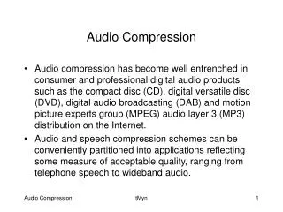
3. Differential pulse code modulation is a derivative of the standard PCM • It uses the fact that the range of differences in amplitudes between successive samples of the audio waveform is less than the range of the actual sample amplitudes • Hence fewer bits to represent the difference signals

4. Operation of DPCM Encoder • Previously digitized sample is held in the register (R) • The DPCM signal is computed by subtracting the current contents (Ro) from the new output by the ADC (PCM) • The register value is then updated before transmission Decoder • Decoder simply adds the previous register contents (PCM) with the DPCM • Since ADC will have noise there will be cumulative errors in the value of the register signal

5. Audio Compression- Third-order predictive DPCM signal encoder and decoder

6. Operation of DPCM • To eliminate this noise effect predictive methods are used to predict a more accurate version of the previous signal (use not only the current signal but also varying proportions of a number of the preceding estimated signals) • These proportions used are known as predictor coefficients • Difference signal is computed by subtracting varying proportions of the last three predicted values from the current output by the ADC

7. Operation of DPCM • R1, R2, R3 will be subtracted from PCM • The values in the R1 register will be transferred to R2 and R2 to R3 and the new predicted value goes into R1 • Decoder operates in a similar way by adding the same proportions of the last three computed PCM signals to the received DPCM signal

8. Adaptive differential PCM (ADPCM) • Savings of bandwidth is possible by varying the number of bits used for the difference signal depending on its amplitude (fewer bits to encode smaller difference signals) • An international standard for this is defined in ITU-T recommendation G721 • This is based on the same principle as the DPCM except an eight-order predictor is used and the number of bits used to quantize each difference is varied • This can be either 6 bits – producing 32 kbps – to obtain a better quality output than with third order DPCM, or 5 bits- producing 16 kbps – if lower bandwidth is more important

9. Audio Compression- ADPCM subband encoder and decoder schematic • The principle of adaptive differential PCM varies the number of bits used for the difference signal depending on its amplitude

10. Adaptive differential PCM (ADPCM) • A second ADPCM standard which is a derivative of G-721 is defined in ITU-T Recommendation G-722 (better sound quality) • This uses subband coding in which the input signal prior to sampling is passed through two filters: one which passes only signal frequencies in the range 50Hz through to 3.5kHz and the other only frequencies in the range 3.5kHz through to 7kHz • By doing this the input signal is effectively divided into two separate equal-bandwidth signals, the first known as the lower subband signal and the second the upper subband signal • Each is then sampled and encoded independently using ADPCM, the sampling rate of the upper subband signal being 16 ksps to allow for the presence of the higher frequency components in this subband

11. Adaptive differential PCM (ADPCM) • The use of two subbands has the advantage that different bit rates can be used for each • In general the frequency components in the lower subband have a higher perceptual importance than those in the higher subband • For example with a bit rate of 64 kbps the lower subband is ADPCM encoded at 48kbps and the upper subband at 16kbps • The two bitstreams are then multiplexed together to produce the transmitted (64 kbps) signal – in such a way that the decoder in the receiver is able to divide them back again into two separate streams for decoding

12. Adaptive predictive coding • Even higher levels of compression possible at higher levels of complexity • These can be obtained by also making the predictor coefficients adaptive • In practice, the optimum set of predictor coefficients continuously vary since they are a function of the characteristics of the audio signal being digitized • To exploit this property, the input speech signal is divided into fixed time segments and, for each segment, the currently prevailing characteristics are determined. • The optimum set of coefficients are then computed and these are used to predict more accurately the previous signal • This type of compression can reduce the bandwidth requirements to 8kbps while still obtaining an acceptable perceived quality

13. Linear predictive coding (LPC) signal encoder and decoder • Linear predictive coding involves the source simply analyzing the audio waveform to determine a selection of the perceptual features it contains

14. Linear predictive coding • With this type of coding the perceptual features of an audio waveform are analysed first • These are then quantized and sent and the destination uses them, together with a sound synthesizer, to regenerate a sound that is perceptually comparable with the source audio signal • With this compression technique although the speech can often sound synthetic high levels of compressions can be achieved • In terms of speech, the three features which determine the perception of a signal by the ear are its: Pitch: this is closely related to the frequency of the signal. This is important since ear is more sensitive to signals in the range 2-5kHz Period: this is the duration of the signal Loudness: This is determined by the amount of energy in the signal

15. Linear predictive coding • The input speech waveform is first sampled and quantized at a defined rate • A block of digitized samples – known as segment - is then analysed to determine the various perceptual parameters of the speech that it contains • The output of the encoder is a string of frames, one for each segment • Each frame contains fields for pitch and loudness – the period determined by the sampling rate being used – a notification of whether the signal is voiced (generated through the vocal cords) or unvoiced (vocal cords are opened) • And a new set of computed modal coefficients

16. Code-excited LPC (CELPC) • The synthesiser used in most LPC decoders are based on a very basic model of the vocal tract • These are intended for use with applications in which the amount of bandwidth available is limited but the perceived quality of the speech must be of acceptable standard for use in various multimedia applications • In CELPC model instead of treating each digitized segment independently for encoding purposes, just a limited set of segments are used, each known as a wave template • A pre computed set of templates are held by the encoder and the decoder in what is known as the template codebook • Each of the individual digitized samples that make up a particular template in the codebook are differently encoded

17. Code-excited LPC (CELPC) • All coders of this type have a delay associated with them which is incurred while each block of digitized samples is analysed by the encoder and the speech is reconstructed at the decoder • The combined delay value is known as the coder’s processing delay • In addition before the speech samples can be analysed it is necessary to buffer the block of samples • The time to accumulate the block of samples is known as the algorithmic delay • The coders delay an important parameter in conventional telephony application, a low-delay coder is required whereas in an interactive application delay of several seconds before the speech starts is acceptable

18. Perceptual Coding (PC) • LPC and CELP are used for telephony applications and hence compression of speech signal • PC are designed for compression of general audio such as that associated with a digital television broadcast • Using this approach, sampled segments of the source audio waveform are analysed – but only those features that are perceptible to the ear are transmitted • E.g although the human ear is sensitive to signals in the range 15Hz to 20 kHz, the level of sensitivity to each signal is non-linear; that is the ear is more sensitive to some signals than others • Also when multiple signals are present as in audio a strong signal may reduce the level of sensitivity of the ear to other signals which are near to it in frequency, an effect known as ‘frequency masking

19. Perceptual Coding (PC) • When the ear hears a loud sound it takes a short but a finite time before it could hear a quieter sound an effect known as temporal masking Sensitivity of the ear • The dynamic range of ear is defined as the loudest sound it can hear to the quietest sound • Sensitivity of the ear varies with the frequency of the signal • The ear is most sensitive to signals in the range 2-5kHz hence the signals in this band are the quietest the ear is sensitive to • Vertical axis gives all the other signal amplitudes relative to this signal (2-5 kHz) • Signal A is above the hearing threshold and B is below the hearing threshold

20. Audio Compression – Perceptual properties of the human ear • Perceptual encoders have been designed for the compression of general audio such as that associated with a digital television broadcast

21. Audio Compression – Perceptual properties of the human ear • When an audio sound consists of multiple frequency signals is present, the sensitivity of the ear changes and varies with the relative amplitude of the signal

22. Perceptual Coding (PC) • Signal B is larger than signal A. This causes the basic sensitivity curve of the ear to be distorted in the region of signal B • Signal A will no longer be heard as it is within the distortion band

23. Audio Compression – Variation with frequency of effect of frequency masking • The width of each curve at a particular signal level is known as the critical bandwidth for that frequency

24. Variation with frequency of effect of frequency masking • The width of each curve at a particular signal level is known as the critical bandwidth • It has been observed that for frequencies less than 500Hz, the critical bandwidth is around 100Hz, however, for frequencies greater than 500Hz then bandwidth increases linearly in multiples of 100Hz • Hence if the magnitude of the frequency components that make up an audio sound can be determined, it becomes possible to determine those frequencies that will be masked and do not therefore need to be transmitted

25. Audio Compression – Temporal masking caused by loud signal • After the ear hears a loud signal, it takes a further short time before it can hear a quieter sound (temporal masking)

26. Temporal masking • After the ear hears a loud sound it takes a further short time before it can hear a quieter sound • This is known as the temporal masking • After the loud sound ceases it takes a short period of time for the signal amplitude to decay • During this time, signals whose amplitudes are less than the decay envelope will not be heard and hence need not be transmitted • In order to achieve this the input audio waveform must be processed over a time period that is comparable with that associated with temporal masking

27. Audio Compression – MPEG perceptual coder schematic

28. MPEG audio coder • The audio input signal is first sampled and quantized using PCM • The bandwidth available for transmission is divided into a number of frequency subbands using a bank of analysis filters • The bank of filters maps each set of 32 (time related) PCM samples into an equivalent set of 32 frequency samples • Processing associated with both frequency and temporal masking is carried out by the psychoacoustic model • In basic encoder the time duration of each sampled segment of the audio input signal is equal to the time to accumulate 12 successive sets of 32 PCM • 12 sets of 32 PCM are converted into frequency components using DFT

29. MPEG audio coder • The output of the psychoacoutic model is a set of what are known as signal-to-mask ratios (SMRs) and indicate the frequency components whose amplitude is below the audible components • This is done to have more bits for highest sensitivity regions compared with less sensitive regions • In an encoder all the frequency components are carried in a frame

30. Audio Compression – MPEG perceptual coder schematic • MPEG audio is used primarily for the compression of general audio and, in particular, for the audio associated with various digital video applications

31. MPEG audio coder frame format • The header contains information such as the sampling frequency that has been used • The quantization is performed in two stages using a form of companding • The peak amplitude level in each subband is first quantized using 6 bits and a further 4 bits are then used to quantize the 12 frequency components in the subband relative to this level • Collectively this is known as the subband sample (SBS) format • The ancillary data field at the end of the frame optional and is used to for example to carry additional coded samples associated with the surround-sound that is present with some digital video broadcasts

32. MPEG audio coder frame format • At the decoder section the dequantizers will determine the magnitude of each signal • The synthesis filters will produce the PCM samples at the decoders

33. Video Compression • One approach to compressing a video source is to apply the JPEG algorithm to each frame independently. This is known as moving JPEG or MJPEG • If a typical movie scene has a minimum duration of 3 seconds, assuming a frame refresh rate of 60 frames/s each scene is composed of 180 frames hence by sending those segments of each frame that has movement associated with them considerable additional savings in bandwidth can be made • There are two types of compressed frames - Those that are compressed independently (I- frames) - Those that are predicted (P-frame and B-frame)

34. Video Compression – Example frame sequences I and P frames • In the context of compression, since video is simply a sequence of digitized pictures, video is also referred to as moving pictures and the terms “frames” and “picture” are used interchangeably

35. Video Compression – I frames • I-frames (Intracoded frames) are encoded without reference to any other frames. Each frame is treated as a separate picture and the Y, Cr and Cb matrices are encoded separately using JPEG • I–frames the compression level is small • They are good for the first frame relating to a new scene in a movie • I-frames must be repeated at regular intervals to avoid losing the whole picture as during transmission it can get corrupted and hence looses the frame • The number of frames/pictures between successive I-frames is known as a group of pictures (GOP). Typical values of GOP are 3 - 12

36. Video Compression – P frames • The encoding of the P-frame is relative to the contents of either a preceding I-frame or a preceding P-frame • P-frames are encoded using a combination of motion estimation and motion compensation • The accuracy of the predictionoperation is determined by how well any movement between successive frames is estimated. This is known as the motion estimation • Since the estimation is not exact, additional information must also be sent to indicate any small differences between the predicted and actual positions of the moving segments involved. This is known as the motion compensation • No of P frames between I-frames is limited to avoid error propagation

37. Video Compression – Frame Sequences I-, P- and B-frames • Each frame is treated as a separate (digitized) picture and the Y, Cb and Cr matrices are encoded independently using the JPEG algorithm (DCT, Quantization, entropy encoding) except that the quantization threshold values that are used are the same for all DCT coefficients

38. Video Compression – PB-Frames • A fourth type of frame known as PB-frame has also been defined; it does not refer to a new frame type as such but rather the way two neighbouring P- and B-frames are encoded as if they were a single frame

39. Video Compression • Motion estimation involves comparing small segments of two consecutive frames for differences and should a difference be detected a search is carried out to determine which neighbouring segments the original segment has moved • To limit the time for search the comparison is limited to few segments • Works well in slow moving applications like video telephony • For fast moving video it will not work effectively. Hence B-frames (Bi-directional) are used. Their contents are predicted using the past and the future frames • B- frames provides highest level of compression and because they are not involved in the coding of other frames they do not propagate errors

40. Video Compression – P-frame encoding • The digitized contents of the Y matrix associated with each frame are first divided into a two-dimensional matrix of 16 X 16 pixels known as a macroblock

41. Video Compression- P-frame encoding • 4 DCT blocks for the luminance signals in the example here and 1 each for the two chrominance signals are used • To encode a p-frame the contents of each macroblock in the frame – known as the target frame are compared on a pixel-by-pixel basis with the contents of the I or P frames (reference frames) • If a close match is found then only the address of the macroblock is encoded • If a match is not found the search is extended to cover an area around the macroblock in the reference frame

42. Video Compression – P-frame encoding • To encode a P-frame, the contents of each macroblock in the frame (target frame) are compared on a pixel-by-pixel basis with the contents of the corresponding macroblock in the preceeding I- or P-frame

43. Video Compression – B-frame encoding • To encode a B-frame, any motion is estimated with reference to both the immediately preceding I- or P-frame and the immediately succeeding P- or I-frame

44. Video Compression- B-frame encoding • To encode B-frame any motion is estimated with reference to both the preceding I or P frame and the succeeding P or I frame • The motion vector and difference matrices are computed using first the preceding frame as the reference frame and then the succeeding frame as the reference • Third motion vectors and set of difference , matrices are then computed using the target and the mean of the two other predicted set of values • The set with the lowest set of difference matrices is chosen and is encoded

45. Decoding of I, P, and B frames • I-frames decode immediately to recreate original frame • P-frames the received information is decoded and the resulting information is used with the decoded contents of the preceding I/P frames (two buffers are used) • B-frames the received information is decoded and the resulting information is used with the decoded contents of the preceding and succeeding P or I frame (three buffers are used) PB-frame • A new frame type showing how two neighbouring P and B frames are encoded as if they were a single frame

46. Video Compression – Implementation schematic – I-frames • The encoding procedure used for the macroblocks that make up an I-frame is the same as that used in the JPEG standard to encode each 8 x 8 block of pixels

47. Implementation Issues • I-frame same as JPEG implementation • FDCT, Quantization, entropy encoding • Assuming 4 blocks for the luminance and 2 blocks for the chrominance, each macroblock would require six 8x8 pixel blocks to be encoded

48. Implementation Issues- P-frames • In the case of P-frames the encoding of each macroblock is dependent on the output of the motion estimation unit which, in turn, depends on the contents of the macroblocks being encoded and the contents of the macroblock in the search area of the reference frame that produces the closest match. There are three possibilities: - If the two contents are the same, only the address of the macroblock in the reference frame is encoded - If the two contents are very close, both the motion vector and the difference matrices associated with the macroblock in the reference frame are encoded - If no close match is found, then the target macroblock is encoded in the same way as a macroblock in an I-frame

49. Video Compression – Implementation schematic – P-frames • In order to carry out its role, the motion estimation unit containing the search logic, utilizes a copy of the (uncoded) reference frame

50. Video Compression – Implementation schematic – B-frames • The same previous procedure is followed for encoding B-frames except both the preceding (reference) and the succeeding frame to the target frame are involved