Download
1 / 68
720 likes | 1.03k Vues
Co-Segmentation. Presented By : Murad Tukan. Introduction. Today there is a massive attempt to exclude the same object from different images. Such problem is not an easy task as it seems , furthermore the algorithm which is presented today is not 100% accurate even though it is efficient.

E N D
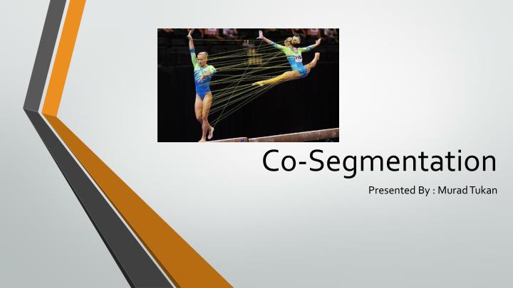
Co-Segmentation Presented By : Murad Tukan
Introduction Today there is a massive attempt to exclude the same object from different images. Such problem is not an easy task as it seems , furthermore the algorithm which is presented today is not 100% accurate even though it is efficient.
What Are We Going To Learn ? An Efficient Algorithm for Co-segmentation . Clothing Co-segmentation for Recognizing People . iCoseg: Interactive Co-segmentation on your iOS device (in short). Implementation of Co-segmentation in MATLAB + C++ Code.
Motivation • The Goal of the Algorithm: • Given a set of images , we need to detect the same foreground in the set of images despite the differences in the background. • Approach : • We will reward consistency in the two foreground histograms.
Images Histogram (Intensity) 1 2
Definitions Co-segmentation settings. Similarity weight. Foreground and background pixels. “MRF penalties”.
Example “image 1”: “image 2”: B1 : B2 :
Foreground and background pixels The segmentation of each image will partition the set of pixel into foreground versus background pixels. Our goal is to ensure that the foreground in the two images are similar.
“MRF penalties” (cont.) • The MRF formulation of one image is then :
Problem Statement (cont.) • Therefore the formulation of co-segmentation problem is then a linear combination of MRF minimization and similarity maximization:
Summarizing We have seen an efficient algorithm, running in polynomial time (the running time of a max-flow algorithm).
Motivation • The goal: • Given a four consumer image collection , we need to recognize individuals among these image collection. • Approach: • Using the clothing data.
Reminders Graph Cut. Normalized Cut. Texture feature vector.
Graph Cut • What are Graph-Cuts ? • Set of edges whose removal makes a graph disconnected. • It’s the partition of V into A,B such that and • A graph can be partitioned into two disjoint sets ,we define the partition cost as: • The bipartition of the graph which minimizes the cut value is called the Min-Cut .
Normalized cut (Ncut) Cut(A,B) is sum of weights with one end in A and one end in B ,we want to minimize the cut cost. Assoc(A,V) is sum of all edges with one end in A , we want to maximize the sum of all weights for every A,B element in the partition
texture feature vector Feature vector based on texture segmentation: We can use spatial filter for where the DOOG filters at various scales and orientations .
Luminance-chrominance space (LCC) The color encoding system used for analog television worldwide (NTSC, PAL and SECAM). The YUV color space (color model) differs from RGB, which is what the camera captures and what humans view. The Y in YUV stands for "luma," which is brightness. U and V provide color information and are "color difference" signals of blue minus luma (B-Y) and red minus luma (R-Y)
Luminance-chrominance space (LCC) (cont.) • RGB to LCC / YUV :
Images and Features for Clothing Analysis • Features are extracted from the faces and clothing of people: • Face features: • Are extracted using an algorithm of detecting face which also can estimate the position of the eyes. • Each face is normalized in scale (49*61 pixels) and projected onto a set of Fisherfaces , representing each face as a 37-dimentional vector.
Fisherfaces • A N x N pixel image of a face, represented as a vector occupies a single point in N2-dimensional image space. • Images of faces being similar in overall configuration, will not be randomly distributed in this huge image space. • Therefore, they can be described by a low dimensional subspace. • Main idea of PCA for faces: • To find vectors that best account for variation of face images in entire image space. • These vectors are called eigen vectors. • Construct a face space and project the images into this face space (eigenfaces).
Images and Features for Clothing Analysis (cont.) • 2: • The 5-dimentional vector at each pixel is quantized to the index of the closest visual word , so each pixel in the region is associated with a word in the dictionary (or several words) then all the words of all the pixels in the region are counted in a histogram. • The Histogram per region is the "feature" of the region. The visual word clothing features are represented as v.
Example of visual words: - red - dots - green … red,dot
Finding the Global Clothing Mask (cont.) The same day mutual information maps are reflected (symmetry is assumed) , summed and thresholded (by a value constant across image collection) to yield clothing masks that appear remarkably similar across collections.