Mathematical Essentials, Probability Concepts, and Statistical Measures

1. Mathematical Essentials, Probability Concepts, and Statistical Measures Steven P. Coy, Ph.D. Continental Airlines AGIFORS Res and YM Study Group Conference, NYC, 2000 AGIFORS Res and YM Study Group Conference, NYC, 2000

2. Mathematical Essentials • A sum of a row or column of n numbers Ex. X = (1, 3, 4, 9) = 1+ 3 + 4 + 9 = 17 • An iterated sum: Sums a matrix of numbers having n rows and j columns • A sequential product of n numbers Ex. X = (1, 3, 4, 9) = 13  4  9 = 108 AGIFORS Res and YM Study Group Conference, NYC, 2000

3. Mathematical Essentials • Convex and concave sets A set of all the points that is bounded by this curve is a convex set A set of all the points that is bounded by this curve is a concave set • In either case, any two points within the set can be connected by a line without leaving the set AGIFORS Res and YM Study Group Conference, NYC, 2000

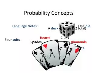
4. Probability Concepts • Experiment • A repeatable procedure • Has a well defined set of possible outcomes • Sample outcome • Potential result of an experiment, denoted e • Sample space • The set of all possible outcomes, denoted S • Event • A subset of the sample space corresponding to the definition of the event, denoted E AGIFORS Res and YM Study Group Conference, NYC, 2000

5. Probability of an Event • Probability is the degree of chance or likelihood that an event will occur in an experiment • Calculating the probability for a discrete or countable problem 1. Find the sum of possible outcomes that satisfy the definition of the event 2. Find the sum of the total number of possible outcomes 3. Divide the result in 1 by the result in 2 • In mathematical notation • P(E) = e  {E} /  e  {S} • P(E)  P(S) = 1 AGIFORS Res and YM Study Group Conference, NYC, 2000

6. Example Experiment: Flip two coins Sample space: {HH, TT, HT, TH} Event: Get at least one head There are three possible outcomes that satisfy E P(E) = 3/4 = .75 Note: P(S) = 1 HT HH TT TH S AGIFORS Res and YM Study Group Conference, NYC, 2000

7. Union and Intersection of Two Events • Intersection • The sum of the sample outcomes of two or more events that are common to all of these events • E1  E2 • Union • The sum of the sample outcomes of two or more events • E1E2 = E1 + E2 - E1  E2 AGIFORS Res and YM Study Group Conference, NYC, 2000

8. Example Experiment: Flip two coins Sample space: {HH, TT, HT, TH} E1 = Get at least one head E2 = Get at least one tail E1  E2 = {TH, HT} E1E2 = S What is P(E1  E2)? What is P(E1  E2)? HT HH TT TH S AGIFORS Res and YM Study Group Conference, NYC, 2000

9. Conditional Probability • Conditional probability is the probability of an event, A, given that a related event, B, has already occurred -- P(A|B) Ex: Draw two cards from a 52-card deck A = draw a Heart as a second card B = draw an Ace as a first card If B = Ace of Hearts, then what is the probability of A given B? Hint: when we draw the Ace of Hearts as a first card, the sample space is effectively reduced by 1 and the number of hearts has been reduced by 1. P(A|B) = 12/51  .24 AGIFORS Res and YM Study Group Conference, NYC, 2000

10. Expectation • Expectation is a long-run average • Example • For some process, P, we must pay $50 every time that we use P. If P is successful, we receive $100, and we know P(S) = .40 (let S denote success) • How much can we expect to make, on average, if we run P? • This requires an expected value computation E(S) = (P(S)  $100) = 40 However. . . E(ROI) = $40 - $50 = -$10 AGIFORS Res and YM Study Group Conference, NYC, 2000

11. Random Variables • Random Variables (RV) are characteristics or outcomes that vary from observation to observation • Independence of two RVs • two RVs are independent if the outcome of one does not affect the outcome of another => P(A|B) = P(A) • Correlation of two random variables • Two RVs are correlated if the knowledge of the outcome of one gives us an indication of the outcome of the other • Positive: X moves with Y • Negative: as X increases, Y decreases AGIFORS Res and YM Study Group Conference, NYC, 2000

12. Probability Distribution of a RV Consider the unconstrained demand for a leisure class ticket on Flt 102: Let’s compile the demand for each departure of Flt 102 for a full year and create a frequency histogram. Notice that the histogram is mound-shaped and approximates a familiar bell-shaped curve. AGIFORS Res and YM Study Group Conference, NYC, 2000

13. Probability Distribution of a Continuous RV • The bell-shaped curve that we saw on the last slide is a normal density curve • Using this chart, we could argue that demand for this flight is normally distributed • Probability calculations with a normal distribution • Example: What is the probability that demand will be less than or equal to 35 pax? • First, we standardize the curve--transform it so that the area under the curve is equal to 1 (we use a z-transform) • We then find the area under the curve that satisfies the definition of our event (the interval 0 to 35) • The area under the curve from 0 to 35 = P(D  35)  .84 AGIFORS Res and YM Study Group Conference, NYC, 2000

14. To find the probability, we find the interval on the horizontal axis and calculate the area under the curve corresponding to that interval (note mean = 30 and std dev = 5) P(D<X)=A AGIFORS Res and YM Study Group Conference, NYC, 2000

15. More About Distributions • Cumulative distribution • In our demand example, we found a probability for a single value of x • A cumulative distribution gives us the probability of D  x for any value of x Cumulative Normal distribution AGIFORS Res and YM Study Group Conference, NYC, 2000

16. Truncated Normal Distribution Demand processes that are described by a normal distribution are truncated at 0--demand cannot be negative AGIFORS Res and YM Study Group Conference, NYC, 2000

17. Demand Unconstraining • We do not always see the “true” distribution of demand since we do not see what was turned away due to class booking limits. • True mean of demand is higher because we are using constrained observations to compute it. • We “unconstrain” demand to find this true mean by looking at the rate of growth in bookings where no limit was reached. This method is not statistically sanctioned. • Expectation Maximization (EM) is a statistical way to unconstrain. Class booking limit = 30 AGIFORS Res and YM Study Group Conference, NYC, 2000

18. Some Common Distributions • Poisson: used to describe the arrival pattern (or process) of people to a system • For example, 5 people request a certain fair class product per hour • Mean = variance • Exponential: used to describe service times • If a process generates poisson arrivals, the generating process has an exponential “service time” • Has special properties that makes it a favorite for queuing systems (waiting lines) and reliability • Uniform (a favorite, because it is easy): the probability is the same throughout • Example U(10, 20): P(x > 15 ) = P(10 < x < 15) AGIFORS Res and YM Study Group Conference, NYC, 2000

19. Statistical Measures • Central tendency • Mean = average • Median = middle value in a sorted list or the middle of a continuous distribution • Mode = largest value or highest portion(s) of a probability density curve • Error measures • e = x - prediction of x • MAD(MAE): Mean absolute deviation (error):  |e| / n • MAPE: Mean absolute percentage error  |e| /x / n AGIFORS Res and YM Study Group Conference, NYC, 2000

20. More Measures • Variance: Measures the dispersion (spread) of the observations • Standard deviation: The square root of the variance • Coefficient of variation: The standard deviation divided by the mean--stated as a percentage • Skew: Measures the asymmetry of a distribution • mean > median: Positive or right-skewed • mean < median: Negative or left-skewed • Correlation: Statistical measure of the relationship between two variables from -1, perfect negative correlation to 1, perfect positive correlation AGIFORS Res and YM Study Group Conference, NYC, 2000