Download
1 / 13
160 likes | 491 Vues
Tirgul 10. Solving parts of the first two theoretical exercises: T1 Q.1(a,b) T1 Q.4(a,e) T2 Q.2(a) T2 Q.3(b) T2 Q.4(a,b). T1 Q.1(a) - pseudo-code for selection sort. Selection-Sort(array A) for j = 0 to A.length - 1 k = smallest(A, j) swap(A, j, k) // swaps A[j] with A[k]

E N D
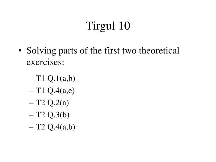
Tirgul 10 • Solving parts of the first two theoretical exercises: • T1 Q.1(a,b) • T1 Q.4(a,e) • T2 Q.2(a) • T2 Q.3(b) • T2 Q.4(a,b)
T1 Q.1(a) - pseudo-code for selection sort Selection-Sort(array A) for j = 0 to A.length - 1 k = smallest(A, j) swap(A, j, k) // swaps A[j] with A[k] return; // Returns the index of the smallest element of A[j..n] int smallest(array A, int j) smallest = j for i = j+1 to A.length - 1 if A[i] < A[smallest] smallest = i return(smallest)
T1 Q.1(b) - proof of correctness • The loop invariant: induction plus “termination claim”. Induction Claim: After performing the j’th iteration, A[0..j-1] contains the j smallest elements in A, sorted in a non-decreasing order: • For j = 1: The algorithm finds the smallest element and places it in A[0] • The induction step: Suppose A[0..j-1] are the j smallest elements. We find the smallest element in A[j..N-1], and thus after the swap A[0..j] are the j+1 smallest elements. Since A[j] is larger than all elements in A[0..j-1] by assumption, then A[0..j] is still sorted. Termination: After n iterations, A[0..n-1] (the entire array) is sorted.
T1 Q.4(a) - solving recurrences • We would like to prove a matching lower bound:
T1 Q.4(e) (another perspective) • How did we guess that T(n) = O(n) ?? • One way is to look at the recursion tree: for any node with work x, the work of all its children is (7/8)x. So the total work of some level is 7/8 times the total work of one level higher, and the first level has work n. So we get an upper bound to the total amount of work:
T2 Q.2(a) - implement queue using two stacks • Denote the two stacks “L” and “R”. • Enqueue: push the item to stack L. • Dequeue: • If stack R is empty: while stack L is not empty, pop an element from stack L and push it to stack R. When stack L is emptied, pop an element from stack R and return it. • If stack R is not empty: pop an element from stack R and return it. • Explanation: 1) If stack R is empty, then after moving the elements from L to R they are in a FIFO order. 2) As long as stack R is not empty, the top element is the first element entered the d.s. (additional enqueus does not change this), so it should be dequeued.
T2 Q.2(a) (continued) • What is the running time? “Most” operations take O(1), occasionally we have O(n) when stack R is empty and we want a dequeue. • If we do amortized analysis (the accounting method) it is enough to pay 3 for every enqueue and 1 for every dequeue, since, after being pushed to stack L, each element has to pay exactly 2 more before being dequeued - 1 for being popped from L and 1 for being pushed to R. • Notice the run-time difference with respect to the more simple solution - always keep the elements in L, and for a dequeue, move the elements to R, return its top, and move the elements back to L. Here, all dequeues are O(n).
T2 Q.3(b) - the selection problem • The selection problem: Given an array A, find the k’th smallest element in linear time (on average). • Reminder from Quicksort: the procdure partition(A,p,r) first chooses a pivot element x from A[p..r], and then rearranges A[p..r] so that all elements before x are smaller than x and all elements after x are larger than x. It returns the new index of x (called q). RandomizedPartition(A,p,r) chooses the pivot randomly. This always takes O(n) time. • What is the size of A[p..q-1] (on average)? If we chose the i’th smallest element then the size will be i-1. Since every element is chosen with probability 1/n then each size 0,..,n-1 has probability 1/n.
T2 Q.3(b) - the algorithm // Returns the k’th element in A[p..r] Select(A, p, r, k) q = RandomizedPartition(A, p, r) if (k == q-p+1) return A[k] else if (k < q-p+1) return Select(A, p, q-1, k) else return Select(A, q+1, r, k-(q-p+1))
T2 Q.3(b) - Average run time • Suppose that the size of A[p..q-1] is i, and k causes us to enter the larger part of A. Since the probability of i is 1/n for i=0..n-1 and the partition takes about n operations: • Assume by induction that T(n) < cn, so (using the arithmetic sum formula):
T2 Q.4 - check the heap property of a given (pointer based) complete binary tree A recursive code: boolean isHeap(Node t) if (t == null) then return TRUE boolean l = isHeap(t.leftChild()) boolean r = isHeap(t.rightChild()) return ( l && r && checkNode(t) ) boolean checkNode(Node t) if ( t.leftChild().val() > t.val() ) return FALSE if ( t.rightChild().val() > t.val() ) return FALSE return TRUE
T2 Q.4 (continued) An iterative code (using a stack): boolean isHeap(Node t) Stack s s.push(t) While ( ! s.empty() ) t = s.pop() if (t != null) if ( ! checkNode(t) ) return FALSE s.push(t.leftChild()) s.push(t.rightChild()) return TRUE