Download
1 / 17
170 likes | 252 Vues
I271B Quantitative Methods. Regression Part I. Administrative Merriments. Next Week: Reading and Evaluating Research Suggest readings using regression, bivariate statistics, etc Course Review May 5 Exam distributed May 7 in class No lecture. Regression versus Correlation.

E N D
I271B Quantitative Methods Regression Part I
Administrative Merriments • Next Week: Reading and Evaluating Research • Suggest readings using regression, bivariate statistics, etc • Course Review May 5 • Exam distributed May 7 in class • No lecture
Regression versus Correlation • Correlation makes no assumption about one whether one variable is dependent on the other– only a measure of general association • Regression attempts to describe a dependent nature of one or more explanatory variables on a single dependent variable. Assumes one-way causal link between X and Y. • Thus, correlation is a measure of the strength of a relationship -1 to 1, while regression is a more precise description of a linear relationship (e.g., the specific slope which is the change in Y given a change in X) • But, correlation is still a part of regression: the square of the correlation coefficient (R2) becomes an expression of how much of Y’s variance is explained by X.
Slope So...what happens if B is negative?
The ‘least squares’ Solution • The distance between each data point and the line of best fit is squared. All of the squared distances are added together. Adapted from Myers, Gamst and Guarino 2006
The Least Squares Solution (cont) • For any Y and X, there is one and only one line of best fit. The least squares regression equation minimizes the possible error between our observed values of Y and our predicted values of Y (often called y-hat). Adapted from Myers, Gamst and Guarino 2006
Important features of regression • There are two regression lines for any bivariate regression • Regression to the mean (regression effect) • Appears whenever there is spread around the SD line (1 SD increase in X r x SDy) • Regression fallacy • Attempting to explain the regression effect through another mechanism
Statistical Inference Using Least Squares • We obtain a sample statistic, b, which estimates the population parameter. • b is the coefficient of the X variable (e.g., how much of a change in the predicted Y is associated with a change in X) • We also have the standard error for b, indicated by e. • We can use a standard t-distribution with n-2 degrees of freedom for hypothesis testing. Yi = b0 + b1xi + ei.
Root Mean Square • Error = actual – predicted • The root-mean-square (r.m.s.) error is how far typical points are above or below the regression line. • Prediction errors are called residuals. • The average of the residuals is = 0. • The S.D. of the residuals is the same as the r.m.s. of the regression line
Interpretation: Predicted Y = constant + (coefficient * Value of X) • For example, suppose we are examining Education (X) in years and Income (Y) in thousands of dollars • Our constant is 10,000 • Our coefficient for X is 5
Heteroskedasticity • OLS regression assumes that the variance of the error term is constant. If the error does not have a constant variance, then it is heteroskedastic (literally, “different scatter”). • Where it comes from • Error may really change as an X increases • Measurement error • Underspecified model
Heteroskedasticity (continued) • Consequences • We still get unbiased parameter estimates, but our line may not be the best fit. • Why? Because OLS gives more ‘weight’ to the cases that might actually have the most error from the predicted line. • Detecting it • We have to look at the residuals (difference between observed responses from the predicted responses) • First, use a residual versus fitted values plot (in STATA, rvfplot) or the residuals versus predicted values plot, which is a plot of the residuals versus one of the independent variables. • We should see an even band across the 0 point (the line), indicating that our error is roughly equal. • If we are still concerned, we can run a test such as the Breusch-Pagan/Cook-Weisberg Test for Heteroskedasticity. It tests the null hypothesis that the error variances are all EQUAL, and the alternative hypothesis that there is some difference. Thus, if it is significant then we reject the null hypothesis and we have a problem of heteroskedasticity.
What to do about Heteroskedasticity? • Perhaps other variables better predict Y? • If you are still interested in current X, you can run a robust regression which will adjust the model to account for heteroskedasticity. • Robust regression modifies the estimates for our standard errors and thus our t-tests for coefficients.
Data points and Regression • http://www.math.csusb.edu/faculty/stanton/m262/regress/
Program and Data for Today: Regress.do GSS96_small.dta