Supply

2. Supply • The analysis of the supply of produced goods has two parts: • An analysis of the supply of the factors of production to households and firms. • An analysis of why firms transform those factors of production into usable goods and services.

3. The Law of Supply • There is a direct relationship between price and quantity supplied. • Quantity supplied rises as price rises, other things constant. • Quantity supplied falls as price falls, other things constant.

4. Law of Supply • Law of Supply • As the price of a product rises, producers will be willing to supply more. • The height of the supply curve at any quantity shows the minimum price necessary to induce producers to supplythat next unit to market. • The height of the supply curve at any quantity also shows the opportunity cost ofproducing the next unitof the good.

5. The Law of Supply • The law of supply is accounted for by two factors: • When prices rise, firms substitute production of one good for another. • Assuming firms’ costs are constant, a higher price means higher profits.

6. The Law of Supply • The law of supply states that there is a positive relationship between price and quantity of a good supplied. • This means that supply curves typically have a positive slope.

7. Supply Schedule • A supply schedule shows how much of a good or service would be supplied at different prices.

8. Supply curve, S Supply Curve Price of coffee beans (per pound) A supply curve shows graphically how much of a good or service people are willing to sell at any given price. $2.00 1.75 As price rises, the quantity supplied rises. 1.50 1.25 1.00 0.75 0.50 0 7 9 11 13 15 17 Quantity of coffee beans (billions of pounds)

9. What Causes a Supply Curve to Shift? • Changes in input prices • An input is a good that is used to produce another good. • Changes in the prices of related goods and services • Changes in technology • Changes in expectations • Changes in the number of producers

10. An Increase in Supply • The entry of Vietnam into the coffee bean business generated an increase in supply—a rise in the quantity supplied at any given price. • This event is represented by the two supply schedules—one showing supply before Vietnam’s entry, the other showing supply after Vietnam came in.

11. S 2 An Increase in Supply Price of coffee beans (per pound) S 1 A shift of the supply curve is a change in the quantity supplied of a good at any given price. $2.00 A movement along the supply curve… 1.75 1.50 1.25 1.00 … is not the same thing as a shift of the supply curve 0.75 0.50 0 7 9 11 13 15 17 Quantity of coffee beans (billions of pounds)

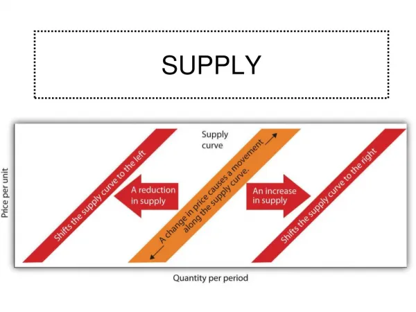
12. Change in price of a good or service leads to Change in quantity supplied(Movement along the curve). Change in costs, input prices, technology, or prices of related goods and services leads to Change in supply (Shift of curve). A Change in Supply Versusa Change in Quantity Supplied To summarize:

13. From Individual Supplyto Market Supply • The supply of a good or service can be defined for an individual firm, or for a group of firms that make up a market or an industry. • Market supply is the sum of all the quantities of a good or service supplied per period by all the firms selling in the market for that good or service.

14. Market Supply • As with market demand, market supply is the horizontal summation of individual firms’ supply curves.

15. Supply, Demand and Equilibrium • Equilibrium in a competitive market: when the quantity demanded of a good equals the quantity supplied of that good. • The price at which this takes place is the equilibrium price (a.k.a. market-clearing price): • Every buyer finds a seller and vice versa. • The quantity of the good bought and sold at that price is the equilibrium quantity.

16. Market Equilibrium • Only in equilibrium is quantity supplied equal to quantity demanded. • At any price level other than P0, the wishes of buyers and sellers do not coincide.

17. Surplus Price of coffee beans (per pound) There is a surplus of a good when the quantity supplied exceeds the quantity demanded. Surpluses occur when the price is above its equilibrium level. Supply $2.00 1.75 Surplus 1.50 1.25 E 1.00 0.75 0.50 Demand 0 7 8.1 10 11.2 13 15 17 Quantity of coffee beans (billions of pounds) Quantity demanded Quantity supplied

18. Shortage Price of coffee beans (per pound) There is a shortage of a good when the quantity demanded exceeds the quantity supplied. Shortages occur when the price is below its equilibrium level. Supply $2.00 1.75 1.50 1.25 E 1.00 0.75 Shortage 0.50 Demand 0 7 9.1 10 11.5 13 15 17 Quantity of coffee beans (billions of pounds) Quantity supplied Quantity demanded

19. Technology Shifts of the Supply Curve S1 Price … leads to a movement along the demand curve to a lower equilibrium price and higher equilibrium quantity. An increase in supply … S2 Technological innovation: In the early 1970s, engineers learned how to put microscopic electronic components onto a silicon chip; progress in the technique has allowed ever more components to be put on each chip. E1 P1 Price falls P2 E2 Demand Quantity Q1 Q2 Quantity increases

20. Market Equilibrium Price of coffee beans (per pound) Market equilibrium occurs at point E, where the supply curve and the demand curve intersect. Supply $2.00 1.75 1.50 1.25 Equilibrium price Equilibrium E 1.00 0.75 0.50 Demand 0 7 10 13 15 17 Quantity of coffee beans (billions of pounds) Equilibrium quantity

21. Equilibrium and Shifts of the Demand Curve Price of coffee beans An increase in demand… Supply … leads to a movement along the supply curve due to a higher equilibrium price and higher equilibrium quantity E 2 P 2 Price rises E 1 P 1 D 2 D 1 Q Q Quantity of coffee beans 1 2 Quantity rises

22. Simultaneous Shifts of Supply and Demand (a) One possible outcome: Price Rises, Quantity Rises Price of coffee Small decrease in supply S S 2 1 Two opposing forces determining the equilibrium quantity. The increase in demand dominates the decrease in supply. E 2 P 2 E 1 P 1 D 2 D 1 Large increase in demand Quantity of coffee Q Q 1 2

23. Simultaneous Shifts of Supply and Demand (b) Another Possibility Outcome: Price Rises, Quantity Falls Price of coffee Large decrease in supply S 2 Two opposing forces determining the equilibrium quantity. S 1 E 2 P 2 E Small increase in demand 1 P 1 D 2 D 1 Q Q Quantity of coffee 2 1

24. Simultaneous Shifts of Supply and Demand We can make the following predictions about the outcome when the supply and demand curves shift simultaneously:

25. Demand and Supply Shifts at Work in the Global Economy • A recent drought in Australia reduced the amount of grass on which Australian dairy cows could feed, thus limiting the amount of milk these cows produced for export. • At the same time, a new tax levied by the government of Argentina raised the price of the milk the country exported, thereby decreasing Argentine milk sales worldwide. • These two developments produced a supply shortage in the world market, which dairy farmers in Europe couldn’t fill because of strict production quotas set by the European Union.

26. Demand and Supply Shifts at Work in the Global Economy • In China, meanwhile, demand for milk and milk products increased, as rising income levels drove higher per-capita consumption. • All these occurrences resulted in a strong upward pressure on the price of milk everywhere in 2007.

27. Section 2-4 Introduction • Whether they are film producers of multimillion-dollar epics or small firms that market a single product, suppliers face a difficult task.  • Producing an economic good or service requires a combination of land, labor, capital, and entrepreneurs.  • The theory of production deals with the relationship between the factors of production and the output of goods and services. Click the mouse button or press the Space Bar to display the information.

28. Section 2-5 Introduction (cont.) • The theory of production generally is based on the short run, a period of production that allows producers to change only the amount of the variable input called labor.  • This contrasts with the long run, a period of production long enough for producers to adjust the quantities of all their resources, including capital. Click the mouse button or press the Space Bar to display the information.

29. Section 2-5 Introduction (cont.) • For example, Ford Motors hiring 300 extra workers for one of its plants is a short-run adjustment.  • If Ford builds a new factory, this is a long-run adjustment. Click the mouse button or press the Space Bar to display the information.

30. Section 2-7 The Production Function (cont.) • Total product is the total output the company produces: a production schedule shows that, as more workers are added, total product rises until a point that adding more workers causes a decline in total product.  • Marginal product is the extra output or change in total product caused by adding one more unit of variable input.

31. Section 2-8 The Production Function (cont.) Click the mouse button or press the Space Bar to display the information.

32. Section 2-9 The Production Function (cont.)

33. Section 2-14 Three Stages of Production • In Stage I, (increasing returns), marginal output increases with each new worker. Companies are tempted to hire more workers, which moves them to Stage II.  • In Stage II, (diminishing returns), total production keeps growing but the rate of increase is smaller; each worker is still making a positive contribution to total output, but it is diminishing. Click the mouse button or press the Space Bar to display the information.

34. Section 2-15 Three Stages of Production (cont.) • In Stage III (negative returns), marginal product becomes negative, decreasing total plant output. Click the mouse button or press the Space Bar to display the information.

35. Overhead is one of many different measures of costs.

36. Section 3-5 Measures of Cost • Fixed costs are those that a business has even if it has no output. These include management salaries, rent, taxes, and depreciation on capital goods.  • Variable costs are those that change when the rate of operation or production changes, including hourly labor, raw materials, freight charges, and electricity. Click the mouse button or press the Space Bar to display the information.

37. Section 3-5 Measures of Cost (cont.) • Total cost is the sum of all fixed costs and all variable costs.  • Marginal cost is the extra (variable) costs incurred when a business produces one additional unit of a product. Click the mouse button or press the Space Bar to display the information.