Download
1 / 35
390 likes | 712 Vues
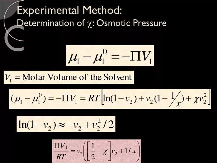
Experimental Method: Determination of : Osmotic Pressure. The osmotic pressure data for cellulose tricaproate in dimethylformamide at three temperatures. The Flory -temperature was determined to be 41 ± 1°C. Modified Flory-Huggins theory. Is temperature dependent.

E N D
The osmotic pressure data for cellulose tricaproate in dimethylformamide at three temperatures. The Flory -temperature was determined to be 41 ± 1°C
Modified Flory-Huggins theory Is temperature dependent Therefore, any temperature which causes =1/2 will be the Flory temperature
Applications of The Chain Expansion Ratio and -Temperature The Expansion Ratio, r
Applications of • ardepends on balance between i) polymer-solvent and ii) polymer-polymer interactions • If (ii) are more favourable than (i) • ar< 1 • Chains contract • Solvent is poor • If (ii) are less favourable than (i) • ar> 1 • Chains expand • Solvent is good • If these interactions are equivalent, we have theta condition • ar = 1 • Same as in amorphous melt
Applications of • For most polymer solutions ardepends on temperature, and increases with increasing temperature • At temperatures above some theta temperature, the solvent is good, whereas below the solvent is poor, i.e., Often polymers will precipitate out of solution, rather than contracting
Applications of The Solvent Goodness: • A Positive A2 indicates a good solvent, i.e. a solvent that gives rise to an exothermic enthalpy of mixing. This arise when <1/2. • When A2=0 the solvent is nearly Ideal. This is important for use of osmotic pressure to measure molar mass. • A negative A2 indicates a poor solvent (>1/2). The entalpy of mixing is positive here. • The goodness of solvent can be adjusted by changing the temperature.
Applications of Recall: Note that the energy terms w11, w22 and w12 are attractive terms and are usually negative . When Hmix=0 for a solvent -polymer system, thus w11=w22 and the cohesive energy density.
Summary Solubility Parameters: Thermodynamics of Mixing
Summary Free Energy of Mixing:
Summary Chemical Potential and Osmotic Pressure:
Summary Other Forms of Flory-Huggins Eqs: 0.35 (in older literature), or zero
Properties of • If the value of is below 0.5, the polymer should be soluble if amorphous and linear. • When equals 0.5, as in the case of the polystyrene–cyclohexane system at 34°C, then the Flory conditions exist. • If the polymer is crystalline, as in the case of polyethylene, it must be heated to near its melting temperature, so that the total free energy of melting plus dissolving is negative. • For very many nonpolar polymer–solvent systems, is in the range of 0.3 to 0.4.
Properties of • For many systems, has been found to increase with polymer concentration and decrease with temperature with a dependence that is approximately linear with, but in general not proportional to, 1/T. • For a given volume fraction 2 of polymer, the smaller the value of , the greater the rate at which the free energy of the solution decreases with the addition of solvent. • Negative values of often indicate strong polar attractions between polymer and solvent.
Properties of • The polymer–solvent interaction parameter is only slightly sensitive to the molecularweight.
Determination of Number Average Mw a) End-group Analysis b) Colligative Properties
Gel Permiation Chromatography Size Exclusion Chromatography
Calibration • GPC is a relative Molecular Weight Method • Narrow molecular weight distribution, anionically polymerized polystyrenes are used most often. • Other Polymers: PMMA, Polyisoprene, polybutadiene, Poly(ethylene oxide) and sodium salts of PMA.