Download
1 / 42
420 likes | 556 Vues
Verification and Calibration of Simulated Reflectivity Products During DWFE. Mark T. Stoelinga University of Washington Thanks to: Steve Koch, NOAA/ESRL/GSD Brad Ferrier, NCEP. Hurricane WRF (Chen 2006, WRF Workshop). 2006 NOAA/SPC Spring Program. WRF-ARW SR. WRF-ARW 3-h Precip.

E N D
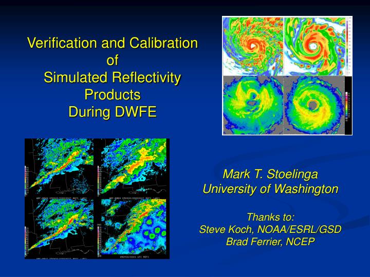
Verification and Calibration of Simulated Reflectivity Products During DWFE Mark T. Stoelinga University of Washington Thanks to: Steve Koch, NOAA/ESRL/GSD Brad Ferrier, NCEP
Hurricane WRF (Chen 2006, WRF Workshop)
WRF-ARW SR WRF-ARW 3-h Precip 2005 DTC Winter Forecast Experiment (DWFE) (Koch et al. 2005) WRF-ARW 700-hPa winds/RH Obs Composite Reflectivity
Forecaster Testimonials “….(we) liked the 4 km BAMEX model run and DON’T want it to go away. The reflectivity forecasts were really very helpful, and almost uncanny.’’ - NWS Forecaster after BAMEX field study “Love the reflectivity product!” - NWS Forecaster after DWFE However,… “Before any meaning can be ascribed to the Reflectivity Product for the purpose of interpreting mesoscale model forecasts, it is important to understand how it is determined.” -Koch et al. (2005) Variational Data Assimilation: What is the best “forward operator” to use as a bridge between observed radar reflectivity and the model microphysics?
Study Goals • Using archived forecast model runs and observed reflectivity from DWFE, examine Simulated Reflectivity (SR) from two different perspectives: • Use statistics and direct examination to see where and why different SR products resemble or differ from observed reflectivity. • Consider the question: If it can be shown that there is a systematic error in a particular SR product, such that the SR product consistently produces too much or too little of a given reflectivity value, can the SR product be “calibrated” to more closely match the observed radar reflectivity?
Data Sources • Archived Gridded Forecast Model Output from DWFE • Archived Observed and Simulated Composite Reflectivity Imagery • 3-D Gridded Observed Reflectivity from the National Mosaic and Multi-Sensor Quantitative Precipitation Estimation (NMQ) Thanks to DTC Thanks to NSSL
13 February 2005 Cyclonic Storm System Stratiform Area Convective/Stratiform Area
Stratiform Area: Composite Reflectivity NMM consistent ARW generic Observed ARW consistent
Stratiform Area: CFADs (Yuter and Houze 1995) Observed ARW generic NMM consistent ARW consistent
Stratiform Area: Frequency Distribution of Height of Maximum Reflectivity 8 6 ARW generic ARW consistent Height above Freezing Level (km) NMM consistent 4 Observed 2 0 -2 0 1000 2000 3000 4000 5000 6000 Number of Occurrences
Differences in ARW Reflectivity Products • Real-time ARW post-processor used a “generic” SR that assumes a constant intercept parameter for the snow size distribution. • “Consistent” ARW SR product uses T-dependent intercept, consistent with WSM5 microphysics in used in ARW. 9 10 10 10 Snow particle size distributions for same mixing ratio qs=0.1 g kg-1 8 10 6 10 8 10 N0 (m-4) N (m-4) 4 10 2 10 7 10 0 10 -2 10 6 -4 10 10 -50 -45 -40 -35 -30 -25 -20 -15 -10 -5 0 0 0.5 1 1.5 2 2.5 3 3.5 4 4.5 5 Temperature (ºC) Particle size (mm)
Differences in ARW Reflectivity Products • Real-time ARW post-processor used a “generic” SR that does not account for the change in dielectric factor for wet snow (“brightband”) • “Consistent” ARW SR product uses the liquid-water dielectric factor for snow that is at T≥ 0 ºC. • → Increases reflectivity by ~7 dBZ in the melting layer
Differences in ARW Reflectivity Products (a) (b) ARW generic ARW generic + var. N0S (b) – (a)
Differences in ARW Reflectivity Products (a) (b) ARW generic + var. N0S ARW generic + var. N0S + wet snow ( = ARW consistent) (b) – (a)
Differences between NMM and ARW Reflectivity Products (a) (b) ARW generic NMM consistent
Stratiform Area: Composite Reflectivity Statistics NMM consistent ARW generic Observed ARW consistent
Stratiform Area: Composite Reflectivity Frequency Distributions 4 10 3 10 Number of grid boxes 2 10 ARW generic 1 ARW consistent 10 NMM consistent Observed 0 10 -20 -10 0 10 20 30 40 50 Reflectivity (dBZ)
Calibration of Composite Simulated Reflectivity Consider the question: If it can be shown that there is a systematic error in a particular SR product, such that the SR product consistently produces too much or too little of a given reflectivity value, can the SR product be “calibrated” to more closely match the observed radar reflectivity? How would we do this? Use the bias? No. SR is too high in some places, too low in others. Use correlation/linear regression? No. Forecast and observed precipitation are not spatially well-correlated. (Ebert and McBride 2000) How about matching the frequency distribution?
Calibration of Composite Simulated Reflectivity 4 10 3 10 Number of grid boxes 2 10 ARW generic 1 ARW consistent 10 NMM consistent Observed 0 10 -20 -10 0 10 20 30 40 50 Reflectivity (dBZ)
Calibration of Composite Simulated Reflectivity We seek a “calibration function” Znew = h(Zm), such that where Zm is the composite SR, and f(Z) and g(Z) are the frequency distributions of the simulated and observed composite reflectivity, respectively.
Calibration of Composite Simulated Reflectivity • While h(Zm) is difficult to extract mathematically, there is a practical and simple way to arrive at it: • Start with a set of SR values that will be used to obtain the calibration equation (e.g., all the grid values of composite SR in a single plot) • Rank all the values in order from lowest to highest value. • Do the same for the corresponding observed reflectivity set. It is important that the same number of points is used for both. • Align the two ranked sets (simulated and observed). The full set of pairs of reflectivity values provide the precise calibration function needed to transform the SR plot into one that has the exact same frequency distribution as the corresponding observed reflectivity plot.
Calibration of Composite Simulated Reflectivity NMM consistent ARW generic Observed ARW consistent
Calibration Curves for Stratiform Area 70 ARW generic 60 ARW consistent NMM consistent 50 40 30 Calibrated Reflectivity (dBZ) 20 10 0 1-to-1 -10 -20 -20 -10 0 10 20 30 40 50 60 70 Simulated Reflectivity (dBZ)
Uncalibrated Composite Simulated Reflectivity NMM consistent ARW generic Observed ARW consistent
Calibrated Composite Simulated Reflectivity (a) (b) NMM consistent ARW generic (c) (d) Observed ARW consistent
13 February 2005 Cyclonic Storm System Stratiform Area Convective/Stratiform Area
Convective/Stratiform Area: Composite Reflectivity NMM consistent ARW generic Observed ARW consistent
Convective/Stratiform Area CFADs Low observed frequency of 20-30dBZ echoes aloft (compared to all models) Observed ARW generic NMM consistent ARW consistent
Convective/Stratiform Area: Frequency Distribution of Height of Maximum Reflectivity 8 6 Height above Freezing Level (km) 4 ARW generic ARW consistent NMM consistent Observed 2 0 -2 0 500 1000 1500 Number of Occurrencess
Convective/Stratiform Area: Composite Reflectivity Frequency Distributions 4 10 3 10 Number of grid boxes 2 10 ARW generic 1 ARW consistent 10 NMM consistent Observed 0 10 -20 -10 0 10 20 30 40 50 Reflectivity (dBZ)
Calibration Curves for Convective/Stratiform Area 70 ARW generic 60 ARW consistent NMM consistent 50 40 30 Calibrated Reflectivity (dBZ) 20 10 0 1-to-1 -10 -20 -20 -10 0 10 20 30 40 50 60 70 Simulated Reflectivity (dBZ)
4-Week Study of Calibration of Composite Simulated Reflectivity What about the mean behavior of the SR products over many different types and intensities of precipitation? 4-week study: 28 February – 24 March 2005 (sub-period of DWFE) Daily forecasts and observations of composite reflectivity at 18, 21, and 00 UTC (18, 21, and 21-h model forecasts) Area covering CONUS from Rocky Mountains eastward Used archived imagery – only 5 dBZ resolution (width of color bands)
4-Week Study of Calibration of Composite Simulated Reflectivity
10 10 10 10 10 10 10 10 4-Week Study of Calibration of Composite Simulated Reflectivity Frequency Distribution 5 4 3 2 Number of pixels 1 ARW generic NMM consistent 0 Observed -1 -2 0 10 20 30 40 50 60 70 Reflectivity (dBZ)
4-Week Study of Calibration of Composite Simulated Reflectivity Calibration Curves 70 60 WRF-ARW (constant N0) WRF-ARW 50 WRF-NMM 40 30 Calibrated Reflectivity (dBZ) 20 10 0 1-to-1 -10 -20 -20 -10 0 10 20 30 40 50 60 70 Simulated Reflectivity (dBZ)
Caveats of SR Calibration • Calibration of SR will not significantly improve correlation of SR and observed reflectivity. • Calibration can only partially compensate for flaws in model microphysics or SR algorithm. • Calibration functions should be based on sufficiently large data sets such that they are not influenced by a small number of bad forecasts, i.e., they should reflect the mean behavior of the model. • Calibration functions are dependent on many factors, including: • - observational data quality • - method of “cartesianizing” the observed reflectivity • - precipitation type • - geographic location and time of year • - model resolution, physics, and forecast hour
Merits of SR Calibration • Calibration can remove systematic under or overprediction of various reflectivity ranges and improve the “look” of SR products. • The process of determining the frequency distribution of SR vs. observed reflectivity, and deriving calibration functions, leads to insights into general flaws in model microphysics and SR algorithms. • Calibration functions may provide a more reasonable “forward operator” for assimilating observed reflectivity data into models than the straight D6 function that is used. • There is potential to enhance the calibration functions, by training them on more limited spatio-temporal windows, or by seeking dependencies on particular types of frequency distributions.
Recommendations • Model microphysics should be formulated not only to optimize QPF, but also to produce reasonable hydrometeor fields and size distributions that affect the model reflectivity. • To the extent possible, SR algorithms should be precisely consistent with all assumptions in the associated model microphysical scheme. • Ideally, SR should be calculated within the model as it runs, to take advantage of the increasingly complex and dynamic size distributions calculated by the schemes. • Real-time or operational SR products should be statistically examined (using CFADs and other frequency distribution tests) to understand how they behave relative to observations. • Real-time or operational SR products should be calibrated with observed reflectivity using the methods described herein. • Calibration functions should be used in forward operators for assimilating reflectivity data into models.