Download
1 / 20
200 likes | 366 Vues
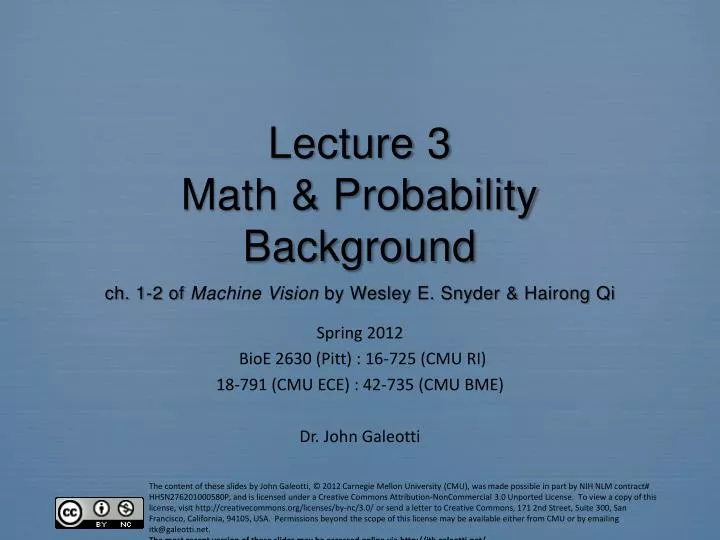
Lecture 3 Math & Probability Background ch. 1-2 of Machine Vision by Wesley E. Snyder & Hairong Qi. Spring 2012 BioE 2630 (Pitt) : 16-725 (CMU RI) 18-791 (CMU ECE) : 42-735 (CMU BME) Dr. John Galeotti. General notes about the book. The book is an overview of many concepts

E N D
Lecture 3Math & Probability Backgroundch. 1-2 of Machine Vision by Wesley E. Snyder & Hairong Qi Spring 2012 BioE 2630 (Pitt) : 16-725 (CMU RI) 18-791 (CMU ECE) : 42-735 (CMU BME) Dr. John Galeotti
General notes about the book • The book is an overview of many concepts • Top quality design requires: • Reading the cited literature • Reading more literature • Experimentation & validation
Two themes • Consistency • A conceptual tool implemented in many/most algorithms • Often must fuse information from local measurements to make global conclusions about the image • Optimization • Mathematical mechanism • The “workhorse” of machine vision
Image Processing Topics • Enhancement • Coding • Compression • Restoration • “Fix” an image • Requires model of image degradation • Reconstruction
Machine Vision Topics Original Image Feature Extraction Classification & Further Analysis • AKA: • Computer vision • Image analysis • Image understanding • Pattern recognition: • Measurement of features Features characterize the image, or some part of it • Pattern classification Requires knowledge about the possible classes Our Focus
Ch. 6-7 Ch. 8 Ch. 9 Ch. 10-11 Ch. 12-16 Feature measurement Original Image Restoration Varies Greatly Noise removal Segmentation Shape Analysis Consistency Analysis Matching Features
Probability • Probability of an event a occurring: • Pr(a) • Independence • Pr(a) does not depend on the outcome of event b, and vice-versa • Joint probability • Pr(a,b) = Prob. of both a and b occurring • Conditional probability • Pr(a|b) = Prob. of a if we already know the outcome of event b • Read “probability of a given b”
Probability for continuously-valued functions • Probability distribution function: P(x) = Pr(z<x) • Probability density function:
Linear algebra • Unit vector: |x| = 1 • Orthogonal vectors: xTy = 0 • Orthonormal: orthogonal unit vectors • Inner product of continuous functions • Orthogonality & orthonormality apply here too
Linear independence • No one vector is a linear combination of the others • xj aixi for any ai across all i j • Any linearly independent set of d vectors {xi=1…d} is a basis set that spans the space d • Any other vector in d may be written as a linear combination of {xi} • Often convenient to use orthonormal basis sets • Projection: if y=aixi then ai=yTxi
Linear transforms • = a matrix, denoted e.g. A • Quadratic form: • Positive definite: • Applies to A if
More derivatives • Of a scalar function of x: • Called the gradient • Really important! • Of a vector function of x • Called the Jacobian • Hessian = matrix of 2nd derivatives of a scalar function
Misc. linear algebra • Derivative operators • Eigenvalues & eigenvectors • Translates “most important vectors” • Of a linear transform (e.g., the matrix A) • Characteristic equation: • A maps x onto itself with only a change in length • is an eigenvalue • x is its corresponding eigenvector
Function minimization • Find the vector x which produces a minimum of some function f (x) • x is a parameter vector • f(x) is a scalar function of x • The “objective function” • The minimum value of f is denoted: • The minimizing value of x is denoted:
Numerical minimization • Gradient descent • The derivative points away from the minimum • Take small steps, each one in the “down-hill” direction • Local vs. global minima • Combinatorial optimization: • Use simulated annealing • Image optimization: • Use mean field annealing
Markov models • For temporal processes: • The probability of something happening is dependent on a thing that just recently happened. • For spatial processes • The probability of something being in a certain state is dependent on the state of something nearby. • Example: The value of a pixel is dependent on the values of its neighboring pixels.
Markov chain • Simplest Markov model • Example: symbols transmitted one at a time • What is the probability that the next symbol will be w? • For a Markov chain: • “The probability conditioned on all of history is identical to the probability conditioned on the last symbol received.”
Hidden Markov models (HMMs) 1st Markov Process f (t) 2nd Markov Process f (t)
HMM switching • Governed by a finite state machine (FSM) Output 1st Process Output 2nd Process
The HMM Task • Given only the output f (t), determine: • The most likely state sequence of the switching FSM • Use the Viterbi algorithm • Computational complexity = (# state changes) * (# state values)2 • Much better than brute force, which = (# state values)(# state changes) • The parameters of each hidden Markov model • Use the iterative process in the book • Better, use someone else’s debugged code that they’ve shared