Download
1 / 193
2k likes | 2.19k Vues
Basic Engineering Mathematics with Matlab. Professor Long-Wen Chang National Tsing Hua University Hsinchu, Taiwan. Why engineering mathematics is very important ? It is very important for the applications of signal analysis. The applications include

E N D
Basic Engineering Mathematics with Matlab Professor Long-Wen Chang National Tsing Hua University Hsinchu, Taiwan
Why engineeringmathematics is very important ? It is very important for the applications of signal analysis. The applications include electrical engineering, computer engineering, civil engineering, mechanical engineering and physics etc..
Outlines • One dimensional continuous time signals • One dimensional continuous systems • Linear ODE in the time domain • The Laplace transform • Linear ODE in the Laplace transform domain • Fourier transform • Analog filters
Why a learning tool is needed ? • To learn efficiently and effectively • To learn by doing simulations
The learning tools • Low cost and high speed multimedia computers are available. • Mathematical Software such as Matlab, Mapel, Mathematica is available. • Microsoft power point is very good for presentation.
Why MATLAB is used ? • It can use a simple instruction to compute a very complex mathematical function. • It provides high resolution two dimensional and three dimensional graphic plot functions for signal analysis.
Why MATLAB is used ? • It can play the sound and display an image in a personal computer or a workstation locally or from the computer network with the X window interface. • MATLAB programs are portable in many computer systems.
Why MATLAB is used ? • It provides interface with the programming language C to enhance its programming ability and execution speed. • We can write a simple program easily to simulate an application which might takes many hours or many days in C or Fortran.
Outline • What are signals ? • What are analog signals ? • What are physical signals ? • Bounded signals with finite energy • Linear convolution of two analog signals
Introduction What are Signals ? In a real world a lot of physical events can be described as signals.
Examples Ultrasound signals are helpful for medicine; Seismic signals are used to detect the earthquake; Electric signals are used to operate electric devices; Radio signals are used for communication.
Examples There are also other signals that are very useful. Among them, audio signals and visual signals are the most important for human beings. Audio signals can be heard while visual signals can be seen.
What are Multimedia signals? • Audio • Video • Image • Text • Graphics
Figure 1.1 shows a sound wave Figure 1.2 shows a mandrill image.
Phantom of Opera • 8 bits, 44.1 Hz (Mono) • '8 bits, 22.05Hz(Mono) • '8 bits, 44.1 Hz(Stereo) • ‘16 bits, 22.05 Hz(Mono)
How to play a .wav file ? • [y,fs]=wavread('adam.wav'); • t=(1:length(y))/fs; • fr=int2str(fs); • plot(t,y); • title(['Sample frequency= ',fr,'(Hz)']); • xlabel('Time'); • sound(y,fs);
Physical Signals In a physical world, signals are real values with finite energy. Mathematical Signals In a mathematical world, signals can be complex valued and have infinite energy.
Definition 1:An one dimensional real-valued analog signal is defined as a piecewise continuous function ,where . Its magnitude is defined as its absolute value
What are analog signals ? Traditionally, analog signals means signals that are continuous in both time and magnitude. Continuous time signals means analog signals.
Analog Signals • Sinusoidal signals • DC signals • Unit step signals • rectangular signals • triangular signals • Exponential signals • square signals
Analog signals (continued) • Sgn(t) • Cosh(t) • Sinh(t) • Sinc(t)
Analog Signals(Continued) • Nonperiodic signals • Periodic signals • Time limited signals • non-time limited signals
Definition 2:Assume that a > 0. A sinusoidal signals is defined as an analog signal (1.1) Where a is the amplitude and is the phase shift and w is the angular frequency given as (1.2)
T is the period of the signal is called the cycle frequency in cycles/second. A cycle per second is also called a hertz (Hz).
How to characterize a sinusoidalsignals? • Amplitude • Frequency • Phase shift
The signal sin(wt + ) is a translated version of sin(wt). Similarly, f(t+a) is a translated version of f(t).
Example 1:The signals a cos(wt) and a sin(wt) are continuous cosine and sine signals. They both have the amplitude a and the frequency w. Figure 1.3(a) and Figure 1.3(b) shows a cosine signal cos(2t) and a sine signal sin(2t). Their frequencies are 1 cycle/sec(Hz) and their amplitudes are 1, respectively. Note that
Similarly, an electric voltage source f(t) = 110 * sin(120*t) has 60 Hz and it maximum voltage is 110 volts. Figure 1.4 shows sin(2t), sin(10t) and sin(20t). Their frequencies are 1 cycle/sec, 5 cycles/sec and 10 cycles/sec,respectively. As the frequency increases the signal oscillates rapidly.
What are the frequencies of thefollowing signals ? • sin(2t) • sin(20t) • sin(20t) • sin(200t) • sin(2000t)
Conventionally, cosine signals and sine signals with nonzero frequency are called AC signals. If their frequencies are large they are referred as high frequency signals; otherwise they are referred as low frequency signals. A signal with zero frequency is called a DC signal.
Continuous plot • % Generate a 1 Hz cosine function sampled by T sec. • T=0.02; • t = -1 :T:1; • y = cos(2 * pi * t); • plot(t,y); xlabel('t'); • ylabel('f(t)');set(gca, 'Ylim',[-2, 2]);
Definition 3:A DC signal is defined as f(t) = c, where cR and -<t< . Figure 1.3(c) shows a DC signal with c = 1 and A DC voltage source can be considered as a sinusoidal voltage source with zero frequency.
Definition 4:An real valued exponential signal is defined as , where aR. Figure 1.5(a) and 1.5(b) shows two exponential signals with a = 1 and a = -1for -1t 1. If a>0 the signal increase exponentially to ; If a < 0 the signal decreases exponentially to 0.
Definition 5:A unit step signal u(t) is defined as (1.3) It has a discontinuity at t = 0. Figure 1.7 shows a unit step signal for -10 t 10.