Download
1 / 52
560 likes | 800 Vues
Orbital Theory of the Ice Ages. Interglacial. Glacial. Milankovitch Theory of the Ice Ages. Milutin Milankovitch (1941) Kanon der Erdbestrahlung und seine Anwendung auf das Eiszeitenproblem (Canon of Insolation of the Earth and Its Application to the Problem of the Ice Ages).

E N D
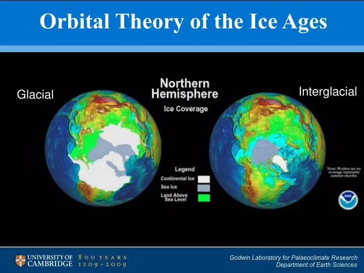
Orbital Theory of the Ice Ages Interglacial Glacial
Milankovitch Theory of the Ice Ages Milutin Milankovitch (1941) Kanon der Erdbestrahlung und seine Anwendung auf das Eiszeitenproblem (Canon of Insolation of the Earth and Its Application to the Problem of the Ice Ages) Forcing: Boreal Summer insolation
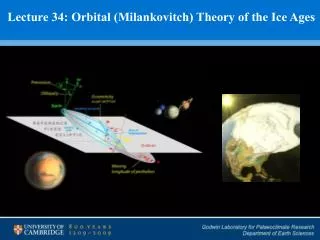
Orbital forcing of Earth’s climate Changes in Earth’s orbital geometry (eccentricity, tilt, precession) Changes in the seasonal distribution of Insolation (heat) as a function of latitude Amplified by other processes Glacial-interglacial climate change
James Croll • Scottish (1821-1890) • Millwright, carpenter, tea shopkeeper, electrical sales, hotelkeeper, insurance salesman, janitor, Geologic Survey, Royal Fellow decreases in winter radiation would favor snow accumulation, coupled this to the idea of a positive ice-albedo feedback to amplify the solar variations.
Milutin Milankovitch, • Serbian mathematician • (1879-1958) • 1941, “Canon of Insolation of the Earth and Its Application to the Problem of the Ice Ages,” 626 pages • improved upon Croll's work partly by using more precise calculations • Emphasized decreases in summer radiation favored snow accumulation and glacial advance
60 65 70 Latitude of equivalent insolation 75 300 250 200 150 100 0 50
Obliquity creates inter-hemispheric heat imbalance (caloric equator shifts seasonally)
Obliquity • Current value: 23.5o • Range: 22o-24.5o • Period: 41,000 yrs
Effect of Obliquity on Insolation difference in obliquity from 22 to 24.5o with other parameters held at present values Effect on insolation is greatest at high latitudes Same sign for respective summer season (hemispheric response is in phase).
varies at a period of 41 kyrs. Obliquity frequency [1/ky] Period [ky] Amplitude 0.02439 40.996 0.011168 0.02522 39.657 0.004401 0.02483 40.270 0.003010 0.01862 53.714 0.002912 0.03462 28.889 0.001452
Eccentricity r r’ Perihelion Aphelion a b Earth travel around the sun in an elliptical orbit with the Sun at one focus
Current value: 0.017 • Range: 0-0.06 • Period(s): ~100,000 yrs ~400,000 yrs
What makes eccentricity vary?The gravitational pull of the other planets • The pull of another • planet is strongest • when the planets • are close together • The net result of • all the mutual inter- • actions between • planets is to vary the • eccentricities of their • orbits
Eccentricity changes the total insolation received by the Earth but the difference is small! 0.5/342.7 = 0.15% Dominant periods are at ~400 and 100 kyrs Eccentricity frequency [1/ky]Period [ky]Amplitude 0.00246406.1820.010851 0.0105594.8300.009208 0.00807123.8820.007078 0.0101498.6070.005925 0.00769130.0190.005295
Precession (axial)
Precession of the axis of the earth Year: Axial Precession
Precession of the Ellipse • Elliptical shape of Earth’s orbit rotates • Precession of ellipse is slower than axial precession • Both motions shift position of the solstices and equinoxes
Precession of the Equinoxes • Earth’s wobble and rotation of its elliptical orbit produce precession of the solstices and equinoxes • One cycles takes 23,000 years • Simplification of complex angular motions in three-dimensional space
Extreme Solstice Positions • Today June 21 solstice is near aphelion (July 4) • Solar radiation a bit lower making summers a bit cooler • Configuration reversed ~11,500 years ago • Precession moves June solstice to perihelion • Solar radiation a bit higher, summers are warmer • Assumes no change in eccentricity
Effect of precession from its minimum value (boreal winter at perihelion) to its maximum value (boreal summer) Precession affects insolation at both high and low latitudes. Opposite sign in northern and southern hemispheres for respective season (out of phase)
Dominant periods at ~19, 22 and 24 kyrs Precession frequency [1/ky]Period [ky]Amplitude 0.0422123.6900.018839 0.0446722.3850.016981 0.0527518.9560.014792 0.0523619.0970.010121 0.0432623.1140.004252
Ice Growth Configuration • (cool summers) • Low obliquity (low seasonal contrast) • High eccentricity and NH summers during aphelion (cold summers in the north)
The equilibrium line of a glacier is the location where winter accumulation of snow is equal to the summer loss. Decreased summer insolation lowers the equilibrium line and glacier advances.
Ice Decay (Deglaciation) • High obliquity (high seasonal contrast) • High eccentricity and NH summers during perihelion (hot summers in the north)
The Forcing: Insolation at 65°N, June 21 Ice decay Ice growth
Milankovitch Theory Revived: The Evidence Shackelton & Opdyke, 1972 Pacific deep core V28-238
Variations in the Earth's Orbit: Pacemaker of the Ice Ages J. D. Hays, John Imbrie, N. J. Shackleton Science, 194, No. 4270, (Dec. 10, 1976), pp. 1121-1132 (eccentricity) (obliquity) (precession) Marine oxygen isotope record shows the same periodicities predicted by orbital forcing.
I II III IV V VI Ice decay Ice growth
Power spectrum of June Insolation at 65oN precession obliquity Note absence of 100 Kyr power
100 ky 41 ky 23 ky Insolation 65oN Benthic 18O
The 100-kyr Problem Classic Milankovitch forcing (might consider alternatives) Forcing small ? big Response Why does the climate system have so much 100-kyr power Traditionally explained by non-linear response involving internal feedbacks.
Non-linear ice volume models invoking threshold response Ice Sheet Growth Lags Summer Insolation
Model 1: Calder (1974) 18O Ice volume V = ice volumei = summer insolation at 65°N i0 = insolation threshold k = kA (accumulation) if i < i0 k = kM (melting) if i > i0 18O (observed) Ice volume Produces some 100-kyr power
Model 2: Imbrie and Imbrie (1980) • Written in dimensionless form (i.e., variables are divided by a scaling value) 18O Ice volume Not observed In climate record (time series might be too short) V = ice volume i = summer insolation at 65°N t = tM if V > i (melting) t = tA otherwise Ice volume 18O
Note weak forcing here due to low eccentricity Response (Imbrie and Imbrie, 1980) forcing Ice volume lags insolation forcing by a constant or varying amount of time.
The “Stage 11” Problem V 5 11 1 9 benthic 18O 7 Ice volume model Imbrie and Imbrie (1980)
Model 3: Paillard (1998) Switching between three states: Interglacial (I) Weak glacial (g) Full glacial (G)
Model 3: Paillard (1998) • Very good agreement with record, both in time and frequency domain. • Weakness?: Highly nonlinear, with a large number of adjustable parameters. • (too easily tweaked?) Ice volume 18O
"Ignoring anthropogenic and other possible sources of variation acting at frequencies higher than one cycle per 19,000 years, this model predicts that the long-term cooling trend which began some 6,000 years ago will continue for the next 23,000 years." (Imbrie and Imbrie, 1980)
The Present Interglacial, How and When Will it End? January 1972, Providence, RI. Organizers George Kukla, Czechoslovakian Academy of Sciences, Prague Robley Matthews, Brown University, Providence A conference summary appeared in Science in October 1972.