Friday, 02 February 2007 William H. Hsu Department of Computing and Information Sciences, KSU

1. Lecture 09 of 42 Decision Trees (Concluded) More on Overfitting Avoidance Friday, 02 February 2007 William H. Hsu Department of Computing and Information Sciences, KSU http://www.cis.ksu.edu/~bhsu Readings: Sections 4.1 – 4.2, Mitchell

2. Lecture Outline • Read Sections 3.6-3.8, Mitchell • Occam’s Razor and Decision Trees • Preference biases versus language biases • Two issues regarding Occam algorithms • Is Occam’s Razor well defined? • Why prefer smaller trees? • Overfitting (akaOvertraining) • Problem: fitting training data too closely • Small-sample statistics • General definition of overfitting • Overfitting prevention, avoidance, and recovery techniques • Prevention: attribute subset selection • Avoidance: cross-validation • Detection and recovery: post-pruning • Other Ways to Make Decision Tree Induction More Robust

3. Occam’s Razor and Decision Trees:Two Issues • Occam’s Razor: Arguments Opposed • size(h) based on H - circular definition? • Objections to the preference bias: “fewer” not a justification • Is Occam’s Razor Well Defined? • Internal knowledge representation (KR) defines which h are “short” - arbitrary? • e.g., single“(Sunny Normal-Humidity)  Overcast  (Rain Light-Wind)” test • Answer: L fixed; imagine that biases tend to evolve quickly, algorithms slowly • Why Short Hypotheses Rather Than Any Other Small H? • There are many ways to define small sets of hypotheses • For any size limit expressed by preference bias, some specification S restricts size(h) to that limit (i.e., “accept trees that meet criterion S”) • e.g., trees with a prime number of nodes that use attributes starting with “Z” • Why small trees and not trees that (for example) test A1, A1, …, A11 in order? • What’s so special about small H based on size(h)? • Answer: stay tuned, more on this in Chapter 6, Mitchell

4. 1,2,3,4,5,6,7,8,9,10,11,12,13,14 [9+,5-] Outlook? Boolean Decision Tree for Concept PlayTennis Sunny 1,2,8,9,11 [2+,3-] 4,5,6,10,14 [3+,2-] Overcast Rain Humidity? Wind? Yes 3,7,12,13 [4+,0-] High Normal Strong Light Temp? No No Yes 1,2,8 [0+,3-] 9,11,15 [2+,1-] 6,14 [0+,2-] 4,5,10 [3+,0-] Hot Mild Cool May fit noise or other coincidental regularities 15 [0+,1-] 9 [1+,0-] No Yes Yes 11 [1+,0-] Overfitting in Decision Trees:An Example • Recall: Induced Tree • Noisy Training Example • Example 15: <Sunny, Hot, Normal, Strong, -> • Example is noisy because the correct label is + • Previously constructed tree misclassifies it • How shall the DT be revised (incremental learning)? • New hypothesis h’ = T’ is expected to perform worse than h = T

5. Overfitting in Inductive Learning • Definition • Hypothesis hoverfits training data set D if  an alternative hypothesis h’ such that errorD(h) < errorD(h’) but errortest(h) > errortest(h’) • Causes: sample too small (decisions based on too little data); noise; coincidence • How Can We Combat Overfitting? • Analogy with computer virus infection, process deadlock • Prevention • Addressing the problem “before it happens” • Select attributes that are relevant (i.e., will be useful in the model) • Caveat: chicken-egg problem; requires some predictive measure of relevance • Avoidance • Sidestepping the problem just when it is about to happen • Holding out a test set, stopping when h starts to do worse on it • Detection and Recovery • Letting the problem happen, detecting when it does, recovering afterward • Build model, remove (prune) elements that contribute to overfitting

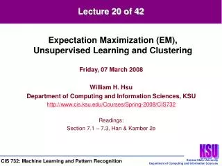
6. 0.9 0.85 0.8 0.75 0.7 0.65 0.6 0.55 0.5 On training data Accuracy On test data 0 10 20 30 40 50 60 70 80 90 100 Size of tree (number of nodes) Decision Tree Learning:Overfitting Prevention and Avoidance • How Can We Combat Overfitting? • Prevention (more on this later) • Select attributes that are relevant (i.e., will be useful in the DT) • Predictive measure of relevance: attribute filter or subset selection wrapper • Avoidance • Holding out a validation set, stopping when hT starts to do worse on it • How to Select “Best” Model (Tree) • Measure performance over training data and separate validation set • Minimum Description Length (MDL): minimize size(h T) + size (misclassifications (h T))

7. Decision Tree Learning:Overfitting Avoidance and Recovery • Today: Two Basic Approaches • Pre-pruning (avoidance): stop growing tree at some point during construction when it is determined that there is not enough data to make reliable choices • Post-pruning (recovery): grow the full tree and then remove nodes that seem not to have sufficient evidence • Methods for Evaluating Subtrees to Prune • Cross-validation: reserve hold-out set to evaluate utility of T (more in Chapter 4) • Statistical testing: test whether observed regularity can be dismissed as likely to have occurred by chance (more in Chapter 5) • Minimum Description Length (MDL) • Additional complexity of hypothesis T greater than that of remembering exceptions? • Tradeoff: coding model versus coding residual error

8. Reduced-Error Pruning • Post-Pruning, Cross-Validation Approach • Split Data into Training and Validation Sets • Function Prune(T, node) • Remove the subtree rooted at node • Make node a leaf (with majority label of associated examples) • Algorithm Reduced-Error-Pruning (D) • Partition D into Dtrain (training / “growing”), Dvalidation(validation / “pruning”) • Build complete tree T using ID3 on Dtrain • UNTIL accuracy on Dvalidation decreases DO FOR each non-leaf node candidate in T Temp[candidate]  Prune (T, candidate) Accuracy[candidate]  Test (Temp[candidate], Dvalidation) T T’  Temp with best value of Accuracy (best increase; greedy) • RETURN (pruned) T

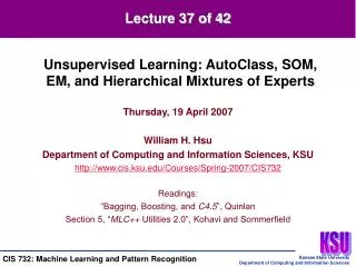
9. On test data Post-pruned tree on test data 0.9 0.85 0.8 0.75 0.7 0.65 0.6 0.55 0.5 On training data Accuracy 0 10 20 30 40 50 60 70 80 90 100 Size of tree (number of nodes) Effect of Reduced-Error Pruning • Reduction of Test Error by Reduced-Error Pruning • Test error reduction achieved by pruning nodes • NB: here, Dvalidation is different from both Dtrain and Dtest • Pros and Cons • Pro: Produces smallest version of most accurate T’ (subtree of T) • Con: Uses less data to construct T • Can afford to hold out Dvalidation? • If not (data is too limited), may make error worse (insufficient Dtrain)

10. Rule Post-Pruning • Frequently Used Method • Popular anti-overfitting method; perhaps most popular pruning method • Variant used in C4.5, an outgrowth of ID3 • Algorithm Rule-Post-Pruning (D) • Infer T from D (using ID3) - grow until D is fit as well as possible (allow overfitting) • Convert T into equivalent set of rules (one for each root-to-leaf path) • Prune (generalize) each rule independently by deleting any preconditions whose deletion improves its estimated accuracy • Sort the pruned rules • Sort by their estimated accuracy • Apply them in sequence on Dtest

11. Outlook? Sunny Overcast Rain Humidity? Wind? Yes High Normal Strong Light No Yes No Yes Converting a Decision Treeinto Rules • Rule Syntax • LHS: precondition (conjunctive formula over attribute equality tests) • RHS: class label • Example • IF (Outlook = Sunny)  (Humidity = High) THEN PlayTennis = No • IF (Outlook = Sunny)  (Humidity = Normal) THEN PlayTennis = Yes • … Boolean Decision Tree for Concept PlayTennis

12. Continuous Valued Attributes • Two Methods for Handling Continuous Attributes • Discretization (e.g., histogramming) • Break real-valued attributes into ranges in advance • e.g., {high Temp > 35º C, med  10º C < Temp  35º C, low  Temp  10º C} • Using thresholds for splitting nodes • e.g., Aa produces subsets Aa and A> a • Information gain is calculated the same way as for discrete splits • How to Find the Split with Highest Gain? • FOR each continuous attribute A Divide examples {x D} according to x.A FOR each ordered pair of values (l, u) of A with different labels Evaluate gain of mid-point as a possible threshold, i.e., DA (l+u)/2, DA > (l+u)/2 • Example • ALength: 10 15 21 28 32 40 50 • Class: -++-++- • Check thresholds: Length 12.5?  24.5?  30?  45?

13. Problem • If attribute has many values, Gain(•) will select it (why?) • Imagine using Date = 06/03/1996 as an attribute! • One Approach: Use GainRatio instead of Gain • SplitInformation: directly proportional to c = | values(A) | • i.e., penalizes attributes with more values • e.g., suppose c1 = cDate = n and c2 = 2 • SplitInformation (A1) = lg(n), SplitInformation (A2) = 1 • If Gain(D, A1) = Gain(D, A2), GainRatio (D, A1) << GainRatio (D, A2) • Thus, preference bias (for lower branch factor) expressed via GainRatio(•) Attributes with Many Values

14. Application Domains • Medical: Temperature has cost $10; BloodTestResult, $150; Biopsy, $300 • Also need to take into account invasiveness of the procedure (patient utility) • Risk to patient (e.g., amniocentesis) • Other units of cost • Sampling time: e.g., robot sonar (range finding, etc.) • Risk to artifacts, organisms (about which information is being gathered) • Related domains (e.g., tomography): nondestructive evaluation • How to Learn A Consistent Tree with Low Expected Cost? • One approach: replace gain by Cost-Normalized-Gain • Examples of normalization functions • [Nunez, 1988]: • [Tan and Schlimmer, 1990]: where w determines importance of cost Attributes with Costs

15. Problem: What If Some Examples Missing Values of A? • Often, values not available for all attributes during training or testing • Example: medical diagnosis • <Fever = true, Blood-Pressure = normal, …, Blood-Test = ?, …> • Sometimes values truly unknown, sometimes low priority (or cost too high) • Missing values in learning versus classification • Training: evaluate Gain (D, A) where for some x D, a value for A is not given • Testing: classify a new example x without knowing the value of A • Solutions: Incorporating a Guess into Calculation of Gain(D, A) [9+, 5-] Outlook Sunny Overcast Rain [2+, 3-] [4+, 0-] [3+, 2-] Missing Data:Unknown Attribute Values

16. Connectionist(Neural Network) Models • Human Brains • Neuron switching time: ~ 0.001 (10-3) second • Number of neurons: ~10-100 billion (1010 – 1011) • Connections per neuron: ~10-100 thousand (104 – 105) • Scene recognition time: ~0.1 second • 100 inference steps doesn’t seem sufficient!  highly parallel computation • Definitions of Artificial Neural Networks (ANNs) • “… a system composed of many simple processing elements operating in parallel whose function is determined by network structure, connection strengths, and the processing performed at computing elements or nodes.” - DARPA (1988) • NN FAQ List: http://www.ci.tuwien.ac.at/docs/services/nnfaq/FAQ.html • Properties of ANNs • Many neuron-like threshold switching units • Many weighted interconnections among units • Highly parallel, distributed process • Emphasis on tuning weights automatically

17. When to Consider Neural Networks • Input: High-Dimensional and Discrete or Real-Valued • e.g., raw sensor input • Conversion of symbolic data to quantitative (numerical) representations possible • Output: Discrete or Real Vector-Valued • e.g., low-level control policy for a robot actuator • Similar qualitative/quantitative (symbolic/numerical) conversions may apply • Data: Possibly Noisy • Target Function: Unknown Form • Result: Human Readability Less Important Than Performance • Performance measured purely in terms of accuracy and efficiency • Readability: ability to explain inferences made using model; similar criteria • Examples • Speech phoneme recognition [Waibel, Lee] • Image classification [Kanade, Baluja, Rowley, Frey] • Financial prediction

18. Hidden-to-Output Unit Weight Map (for one hidden unit) Input-to-Hidden Unit Weight Map (for one hidden unit) Autonomous Learning Vehiclein a Neural Net (ALVINN) • Pomerleau et al • http://www.cs.cmu.edu/afs/cs/project/alv/member/www/projects/ALVINN.html • Drives 70mph on highways

19. Perceptron: Single Neuron Model • akaLinear Threshold Unit (LTU) or Linear Threshold Gate (LTG) • Net input to unit: defined as linear combination • Output of unit: threshold (activation) function on net input (threshold = w0) • Perceptron Networks • Neuron is modeled using a unit connected by weighted linkswi to other units • Multi-Layer Perceptron (MLP): next lecture x0= 1 x1 w1 w0 x2 w2 xn wn The Perceptron 

20. x2 x2 + + - + - + x1 x1 - + - - Example A Example B Decision Surface of a Perceptron • Perceptron: Can Represent Some Useful Functions • LTU emulation of logic gates (McCulloch and Pitts, 1943) • e.g., What weights represent g(x1, x2) = AND(x1, x2)? OR(x1, x2)? NOT(x)? • Some Functions Not Representable • e.g., not linearly separable • Solution: use networks of perceptrons (LTUs)

21. Learning Rule  Training Rule • Not specific to supervised learning • Context: updating a model • Hebbian Learning Rule (Hebb, 1949) • Idea: if two units are both active (“firing”), weights between them should increase • wij = wij + r oi oj where r is a learning rate constant • Supported by neuropsychological evidence • Perceptron Learning Rule (Rosenblatt, 1959) • Idea: when a target output value is provided for a single neuron with fixed input, it can incrementally update weights to learn to produce the output • Assume binary (boolean-valued) input/output units; single LTU • where t = c(x) is target output value, o is perceptron output, r is small learning rate constant (e.g., 0.1) • Can prove convergence if Dlinearly separable and r small enough Learning Rules for Perceptrons

22. Understanding Gradient Descent for Linear Units • Consider simpler, unthresholded linear unit: • Objective: find “best fit” to D • Approximation Algorithm • Quantitative objective: minimize error over training data set D • Error function: sum squared error (SSE) • How to Minimize? • Simple optimization • Move in direction of steepest gradient in weight-error space • Computed by finding tangent • i.e. partial derivatives (of E) with respect to weights (wi) Gradient Descent:Principle

23. Terminology • Occam’s Razor and Decision Trees • Preference biases: captured by hypothesis space search algorithm • Language biases : captured by hypothesis language (search space definition) • Overfitting • Overfitting: h does better than h’ on training data and worse on test data • Prevention, avoidance, and recovery techniques • Prevention: attribute subset selection • Avoidance: stopping (termination) criteria, cross-validation, pre-pruning • Detection and recovery: post-pruning (reduced-error, rule) • Other Ways to Make Decision Tree Induction More Robust • Inequality DTs (decision surfaces): a way to deal with continuous attributes • Information gain ratio: a way to normalize against many-valued attributes • Cost-normalized gain: a way to account for attribute costs (utilities) • Missing data: unknown attribute values or values not yet collected • Feature construction: form of constructive induction; produces new attributes • Replication: repeated attributes in DTs

24. Summary Points • Occam’s Razor and Decision Trees • Preference biases versus language biases • Two issues regarding Occam algorithms • Why prefer smaller trees? (less chance of “coincidence”) • Is Occam’s Razor well defined? (yes, under certain assumptions) • MDL principle and Occam’s Razor: more to come • Overfitting • Problem: fitting training data too closely • General definition of overfitting • Why it happens • Overfitting prevention, avoidance, and recovery techniques • Other Ways to Make Decision Tree Induction More Robust • Next Week: Perceptrons, Neural Nets (Multi-Layer Perceptrons), Winnow