Download
1 / 51
510 likes | 713 Vues
CPSC 321 Computer Architecture and Engineering Lecture 8 Designing a Multicycle Processor. Instructor: Rabi Mahapatra & Hank Walker Adapted from the lecture notes of John Kubiatowicz (UCB). Recap: A Single Cycle Datapath. Instruction<31:0>. nPC_sel. Instruction Fetch Unit. Rd. Rt.

E N D
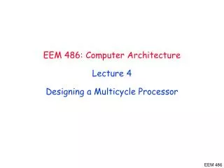
CPSC 321Computer Architecture and EngineeringLecture 8 Designing a Multicycle Processor Instructor: Rabi Mahapatra & Hank Walker Adapted from the lecture notes of John Kubiatowicz (UCB)
Recap: A Single Cycle Datapath Instruction<31:0> nPC_sel Instruction Fetch Unit Rd Rt <21:25> <16:20> <11:15> <0:15> Clk RegDst 1 0 Mux Rs Rt Rd Imm16 Rs Rt RegWr ALUctr 5 5 5 MemtoReg busA Equal MemWr Rw Ra Rb busW 32 32 32-bit Registers 0 ALU 32 busB 32 0 Clk Mux 32 Mux 32 1 WrEn Adr 1 Data In 32 Data Memory Extender imm16 32 16 Clk ALUSrc ExtOp
RegDst func ALUSrc ALUctr ALU Control (Local) op 6 Main Control : 3 6 ALUop 3 op 00 0000 00 1101 10 0011 10 1011 00 0100 00 0010 R-type ori lw sw beq jump RegDst 1 0 0 x x x ALUSrc 0 1 1 1 0 x MemtoReg 0 0 1 x x x RegWrite 1 1 1 0 0 0 MemWrite 0 0 0 1 0 0 Branch 0 0 0 0 1 0 Jump 0 0 0 0 0 1 ExtOp x 0 1 1 x x ALUop (Symbolic) “R-type” Or Add Add xxx Subtract ALUop <2> 1 0 0 0 x 0 ALUop <1> 0 1 0 0 x 0 ALUop <0> 0 0 0 0 x 1 Recap: The “Truth Table” for the Main Control
. . . . . . op<5> op<5> op<5> op<5> op<5> op<5> . . . . . . <0> <0> <0> <0> <0> op<0> R-type ori lw sw beq jump RegWrite ALUSrc RegDst MemtoReg MemWrite Branch Jump ExtOp ALUop<2> ALUop<1> ALUop<0> Recap: PLA Implementation of the Main Control
Recap: Systematic Generation of Control OPcode Control Logic / Store (PLA, ROM) • In our single-cycle processor, each instruction is realized by exactly one control command or “microinstruction” • in general, the controller is a finite state machine • microinstruction can also control sequencing (see later) Decode microinstruction Conditions Instruction Control Points Datapath
The Big Picture: Where are We Now? • The Five Classic Components of a Computer • Today’s Topic: Designing the Datapath for the Multiple Clock Cycle Datapath Processor Input Control Memory Datapath Output
Abstract View of our single cycle processor Main Control op • looks like a FSM with PC as state ALU control fun ALUSrc Equal ExtOp MemWr MemWr MemRd RegWr RegDst nPC_sel ALUctr Reg. Wrt ALU Register Fetch Ext Mem Access PC Instruction Fetch Next PC Result Store Data Mem
What’s wrong with our CPI=1 processor? Arithmetic & Logical PC Inst Memory Reg File ALU setup • Long Cycle Time • All instructions take as much time as the slowest • Real memory is not as nice as our idealized memory • cannot always get the job done in one (short) cycle mux mux Load PC Inst Memory Reg File ALU Data Mem setup mux mux Critical Path Store PC Inst Memory Reg File ALU Data Mem mux Branch PC Inst Memory Reg File cmp mux
storage element Acyclic Combinational Logic storage element Reducing Cycle Time • Cut combinational dependency graph and insert register / latch • Do same work in two fast cycles, rather than one slow one • May be able to short-circuit path and remove some components for some instructions! storage element Acyclic Combinational Logic (A) storage element Acyclic Combinational Logic (B) storage element
Basic Limits on Cycle Time • Next address logic • PC <= branch ? PC + offset : PC + 4 • Instruction Fetch • InstructionReg <= Mem[PC] • Register Access • A <= R[rs] • ALU operation • R <= A + B Control MemWr MemWr MemRd RegWr RegDst nPC_sel ALUctr ALUSrc ExtOp Reg. File Exec Operand Fetch Instruction Fetch Mem Access PC Next PC Result Store Data Mem
Equal Partitioning the CPI=1 Datapath • Add registers between smallest steps • Place enables on all registers MemWr MemWr MemRd RegWr RegDst nPC_sel ALUSrc ExtOp ALUctr Reg. File Exec Operand Fetch Instruction Fetch Mem Access PC Next PC Result Store Data Mem
MemToReg RegWr RegDst MemRd MemWr ALUctr ALUSrc ExtOp Reg. File Ext ALU S Mem Access M Data Mem Result Store Example Multicycle Datapath • Critical Path ? Equal nPC_sel E Reg File A PC IR Next PC B Instruction Fetch Operand Fetch
Recall: Step-by-step Processor Design Step 1: ISA => Logical Register Transfers Step 2: Components of the Datapath Step 3: RTL + Components => Datapath Step 4: Datapath + Logical RTs => Physical RTs Step 5: Physical RTs => Control
Time A S B M Step 4: R-type (add, sub, . . .) inst Logical Register Transfers ADDU R[rd] <– R[rs] + R[rt]; PC <– PC + 4 • Logical Register Transfer • Physical Register Transfers inst Physical Register Transfers IR <– MEM[pc] ADDU A<– R[rs]; B <– R[rt] S <– A + B R[rd] <– S; PC <– PC + 4 E Reg. File Reg File Exec PC IR Next PC Inst. Mem Mem Access Data Mem
Time A S M Step 4: Logical immed inst Logical Register Transfers ORI R[rt] <– R[rs] OR ZExt(Im16); PC <– PC + 4 • Logical Register Transfer • Physical Register Transfers inst Physical Register Transfers IR <– MEM[pc] ORI A<– R[rs]; B <– R[rt] S <– A or ZExt(Im16) R[rt] <– S; PC <– PC + 4 E Reg. File Reg File Exec PC IR Next PC Inst. Mem B Mem Access Data Mem
inst Physical Register Transfers IR <– MEM[pc] LW A<– R[rs]; B <– R[rt] S <– A + SExt(Im16) M <– MEM[S] R[rd] <– M; PC <– PC + 4 Time A S M Step 4 : Load inst Logical Register Transfers LW R[rt] <– MEM[R[rs] + SExt(Im16)]; PC <– PC + 4 • Logical Register Transfer • Physical Register Transfers E Reg. File Reg File Exec PC IR Next PC Inst. Mem B Mem Access Data Mem
Time A S M Step 4 : Store inst Logical Register Transfers SW MEM[R[rs] + SExt(Im16)] <– R[rt]; PC <– PC + 4 • Logical Register Transfer • Physical Register Transfers inst Physical Register Transfers IR <– MEM[pc] SW A<– R[rs]; B <– R[rt] S <– A + SExt(Im16); MEM[S] <– B PC <– PC + 4 E Reg. File Reg File Exec PC IR Next PC Inst. Mem B Mem Access Data Mem
Time S M Step 4 : Branch inst Logical Register Transfers BEQ if R[rs] == R[rt] then PC <= PC + 4+SExt(Im16) || 00 else PC <= PC + 4 • Logical Register Transfer • Physical Register Transfers inst Physical Register Transfers IR <– MEM[pc] BEQE<– (R[rs] = R[rt]) if !E then PC <– PC + 4 else PC <–PC+4+SExt(Im16)||00 E Reg. File Reg File A Exec PC IR Next PC Inst. Mem B Mem Access Data Mem
Target 32 0 Mux 0 Mux 1 0 1 Mux 32 1 ALU Control Mux 1 0 << 2 Extend 16 Alternative datapath (book): Multiple Cycle Datapath PCWr PCWrCond PCSrc BrWr • Miminizes Hardware: 1 memory, 1 adder Zero ALUSelA IorD MemWr IRWr RegDst RegWr 1 Mux 32 PC 0 Zero 32 Rs Ra 32 RAdr 5 32 Rt Rb busA 32 ALU Ideal Memory 32 Reg File 5 32 Instruction Reg ALU Out 4 Rt 0 Rw 32 WrAdr 32 1 32 Rd Din Dout busW busB 32 2 32 3 Imm 32 ALUOp ExtOp MemtoReg ALUSelB
Our Control Model • State specifies control points for Register Transfer • Transfer occurs upon exiting state (same falling edge) inputs (conditions) Next State Logic State X Register Transfer Control Points Control State Depends on Input Output Logic outputs (control points)
Execute Memory Write-back Step 4 Control Specification for multicycle proc “instruction fetch” IR <= MEM[PC] “decode / operand fetch” A <= R[rs] B <= R[rt] LW R-type ORi SW BEQ PC <= Next(PC,Equal) S <= A fun B S <= A or ZX S <= A + SX S <= A + SX M <= MEM[S] MEM[S] <= B PC <= PC + 4 R[rd] <= S PC <= PC + 4 R[rt] <= S PC <= PC + 4 R[rt] <= M PC <= PC + 4
Traditional FSM Controller next state state op cond control points Truth Table next State control points 11 Equal 6 State 4 op datapath State
Step 5 (datapath + state diagram control) • Translate RTs into control points • Assign states • Then go build the controller
Execute Memory Write-back Mapping RTs to Control Points IR <= MEM[PC] “instruction fetch” imem_rd, IRen A <= R[rs] B <= R[rt] “decode” Aen, Ben, Een LW R-type ORi SW BEQ S <= A fun B PC <= Next(PC,Equal) S <= A or ZX S <= A + SX S <= A + SX ALUfun, Sen M <= MEM[S] MEM[S] <= B PC <= PC + 4 R[rd] <= S PC <= PC + 4 RegDst, RegWr, PCen R[rt] <= S PC <= PC + 4 R[rt] <= M PC <= PC + 4
Execute Memory Write-back Assigning States “instruction fetch” IR <= MEM[PC] 0000 “decode” A <= R[rs] B <= R[rt] 0001 LW R-type ORi SW BEQ PC <= Next(PC) S <= A fun B S <= A or ZX S <= A + SX S <= A + SX 0100 0110 1000 1011 0011 M <= MEM[S] MEM[S] <= B PC <= PC + 4 1001 1100 R[rd] <= S PC <= PC + 4 R[rt] <= S PC <= PC + 4 R[rt] <= M PC <= PC + 4 0101 0111 1010
(Mostly) Detailed Control Specification (missing0) State Op field Eq Next IR PC Ops Exec Mem Write-Back en sel A B E Ex Sr ALU S R W M M-R Wr Dst 0000 ?????? ? 0001 1 0001 BEQ x 0011 1 1 1 0001 R-type x 0100 1 1 1 0001 ORI x 0110 1 1 1 0001 LW x 1000 1 1 1 0001 SW x 1011 1 1 1 0011 xxxxxx 0 0000 1 0 x 0 x 0011 xxxxxx 1 0000 1 1 x 0 x 0100 xxxxxx x 0101 0 1 fun 1 0101 xxxxxx x 0000 1 0 0 1 1 0110 xxxxxx x 0111 0 0 or 1 0111 xxxxxx x 0000 1 0 0 1 0 1000 xxxxxx x 1001 1 0 add 1 1001 xxxxxx x 1010 1 0 1 1010 xxxxxx x 0000 1 0 1 1 0 1011 xxxxxx x 1100 1 0 add 1 1100 xxxxxx x 0000 1 0 0 1 0 -all same in Moore machine BEQ: R: ORi: LW: SW:
Performance Evaluation • What is the average CPI? • state diagram gives CPI for each instruction type • workload gives frequency of each type Type CPIi for type Frequency CPIi x freqIi Arith/Logic 4 40% 1.6 Load 5 30% 1.5 Store 4 10% 0.4 branch 3 20% 0.6 Average CPI: 4.1
sequencer control datapath control microinstruction micro-PC sequencer Controller Design • The state digrams that arise define the controller for an instruction set processor are highly structured • Use this structure to construct a simple “microsequencer” • Control reduces to programming this very simple device microprogramming
Example: Jump-Counter i i 0000 i+1 Map ROM None of above: Do nothing (for wait states) op-code zero inc load Counter
Execute Memory Write-back Using a Jump Counter “instruction fetch” IR <= MEM[PC] 0000 inc “decode” A <= R[rs] B <= R[rt] 0001 load LW R-type ORi SW BEQ PC <= Next(PC) S <= A fun B S <= A or ZX S <= A + SX S <= A + SX 0100 0110 1000 1011 0011 inc inc inc inc zero M <= MEM[S] MEM[S] <= B PC <= PC + 4 1001 1100 inc R[rd] <= S PC <= PC + 4 R[rt] <= S PC <= PC + 4 R[rt] <= M PC <= PC + 4 zero 0101 0111 1010 zero zero zero
Our Microsequencer taken datapath control Z I L Micro-PC op-code Map ROM
Microprogram Control Specification µPC Taken Next IR PC Ops Exec Mem Write-Back en sel A B Ex Sr ALU S R W M M-R Wr Dst 0000 ? inc 1 0001 0 load 1 1 0011 0 zero 1 0 0011 1 zero 1 1 0100 x inc 0 1 fun 1 0101 x zero 1 0 0 1 1 0110 x inc 0 0 or 1 0111 x zero 1 0 0 1 0 1000 x inc 1 0 add 1 1001 x inc 1 0 1 1010 x zero 1 0 1 1 0 1011 x inc 1 0 add 1 1100 x zero 1 0 0 1 0 BEQ R: ORi: LW: SW:
Adding the Dispatch ROM • Sequencer-based control unit from last lecture • Called “microPC” or “µPC” vs. state register Control Value Effect00 Next µaddress = 0 01 Next µaddress = dispatch ROM 10 Next µaddress = µaddress + 1 ROM: 1 microPC Adder R-type 000000 0100 BEQ 000100 0011 ori 001101 0110 LW 100011 1000 SW 101011 1011 Mux 2 1 0 0 µAddress Select Logic ROM Opcode
Example: Controlling Memory PC addr InstMem_rd Instruction Memory IM_wait data Inst. Reg IR_en
Execute Memory Write-back Controller handles non-ideal memory “instruction fetch” IR <= MEM[PC] wait ~wait “decode / operand fetch” A <= R[rs] B <= R[rt] LW R-type ORi SW BEQ PC <= Next(PC) S <= A fun B S <= A or ZX S <= A + SX S <= A + SX M <= MEM[S] MEM[S] <= B ~wait wait wait ~wait R[rd] <= S PC <= PC + 4 R[rt] <= S PC <= PC + 4 R[rt] <= M PC <= PC + 4 PC <= PC + 4
Overview of Control • Control may be designed using one of several initial representations. The choice of sequence control, and how logic is represented, can then be determined independently; the control can then be implemented with one of several methods using a structured logic technique. Initial Representation Finite State Diagram Microprogram Sequencing Control Explicit Next State Microprogram counter Function + Dispatch ROMs Logic Representation Logic Equations Truth Tables Implementation PLA ROM Technique “hardwired control” “microprogrammed control”
Microprogramming (Maurice Wilkes) • Control is the hard part of processor design ° Datapath is fairly regular and well-organized ° Memory is highly regular ° Control is irregular and global Microprogramming: -- A Particular Strategy for Implementing the Control Unit of a processor by "programming" at the level of register transfer operations Microarchitecture: -- Logical structure and functional capabilities of the hardware as seen by the microprogrammer Historical Note: IBM 360 Series first to distinguish between architecture & organization Same instruction set across wide range of implementations, each with different cost/performance
“Macroinstruction” Interpretation User program plus Data this can change! Main Memory ADD SUB AND . . . one of these is mapped into one of these DATA execution unit AND microsequence e.g., Fetch Calc Operand Addr Fetch Operand(s) Calculate Save Answer(s) CPU control memory
New Finite State Machine (FSM) Spec IR <= MEM[PC] PC <= PC + 4 “instruction fetch” 0000 “decode” Q: How improve to do something in state 0001? 0001 LW BEQ R-type ORi SW ALUout <= A fun B ALUout <= A or ZX ALUout <= A + SX ALUout <= A + SX ALUout <= PC +SX Execute 0100 0110 1000 1011 0010 M <= MEM[ALUout] MEM[ALUout] <= B Memory If A = B then PC <= ALUout 1001 1100 0011 R[rd] <= ALUout R[rt] <= ALUout R[rt] <= M Write-back 0101 0111 1010
Finite State Machine (FSM) Spec IR <= MEM[PC] PC <= PC + 4 “instruction fetch” 0000 ALUout <= PC +SX “decode” 0001 LW BEQ R-type ORi SW ALUout <= A fun B ALUout <= A or ZX ALUout <= A + SX ALUout <= A + SX If A = B then PC <= ALUout Execute 0100 0110 1000 1011 0010 M <= MEM[ALUout] MEM[ALUout] <= B Memory 1001 1100 R[rd] <= ALUout R[rt] <= ALUout R[rt] <= M Write-back 0101 0111 1010
sequencer control datapath control Inputs microinstruction () -sequencer: fetch,dispatch, sequential micro-PC Decode Decode To DataPath Dispatch ROM Opcode Microprogramming -Code ROM • Microprogramming is a fundamental concept • implement an instruction set by building a very simple processor and interpreting the instructions • essential for very complex instructions and when few register transfers are possible • overkill when ISA matches datapath 1-1
Designing a Microinstruction Set 1) Start with list of control signals 2) Group signals together that make sense (vs. random): called “fields” 3) Place fields in some logical order (e.g., ALU operation & ALU operands first and microinstruction sequencing last) 4) To minimize the width, encode operations that will never be used at the same time 5) Create a symbolic legend for the microinstruction format, showing name of field values and how they set the control signals • Use computers to design computers
32 0 Mux 0 Mux 1 Instruction Reg 32 ALU Out 0 1 Mux 32 32 1 ALU Control Mux 1 0 << 2 Extend 16 Again: Alternative multicycle datapath (book) PCWr PCWrCond PCSrc • Miminizes Hardware: 1 memory, 1 adder Zero ALUSelA IorD MemWr IRWr RegDst RegWr 1 Mux 32 PC 0 Zero 32 Rs Ra 32 RAdr 5 32 Rt 32 Rb busA A ALU Ideal Memory 32 Reg File 5 4 Rt 0 Rw 32 WrAdr 32 B 1 32 Rd Mem Data Reg Din Dout busW busB 2 32 3 Imm 32 ALUOp ExtOp MemtoReg ALUSelB
1&2) Start with list of control signals, grouped into fields Signal name Effect when deasserted Effect when assertedALUSelA 1st ALU operand = PC 1st ALU operand = Reg[rs]RegWrite None Reg. is written MemtoReg Reg. write data input = ALU Reg. write data input = memory RegDst Reg. dest. no. = rt Reg. dest. no. = rdMemRead None Memory at address is read, MDR <= Mem[addr]MemWrite None Memory at address is written IorD Memory address = PC Memory address = SIRWrite None IR <= MemoryPCWrite None PC <= PCSourcePCWriteCond None IF ALUzero then PC <= PCSourcePCSource PCSource = ALU PCSource = ALUoutExtOp Zero Extended Sign Extended Single Bit Control Signal name Value EffectALUOp 00 ALU adds 01 ALU subtracts 10 ALU does function code 11 ALU does logical OR ALUSelB 00 2nd ALU input = 4 01 2nd ALU input = Reg[rt] 10 2nd ALU input = extended,shift left 2 11 2nd ALU input = extended Multiple Bit Control
3&4) Microinstruction Format: unencoded vs. encoded fields Field Name Width Control Signals Set wide narrow ALU Control 4 2 ALUOp SRC1 2 1 ALUSelA SRC2 5 3 ALUSelB, ExtOp ALU Destination 3 2 RegWrite, MemtoReg, RegDst Memory 3 2 MemRead, MemWrite, IorD Memory Register 1 1 IRWrite PCWrite Control 3 2 PCWrite, PCWriteCond, PCSource Sequencing 3 2 AddrCtl Total width 24 15 bits
5) Legend of Fields and Symbolic Names Field Name Values for Field Function of Field with Specific ValueALU Add ALU adds Subt. ALU subtracts Func code ALU does function code Or ALU does logical ORSRC1 PC 1st ALU input = PC rs 1st ALU input = Reg[rs]SRC2 4 2nd ALU input = 4 Extend 2nd ALU input = sign ext. IR[15-0] Extend0 2nd ALU input = zero ext. IR[15-0] Extshft 2nd ALU input = sign ex., sl IR[15-0] rt 2nd ALU input = Reg[rt]destination rd ALU Reg[rd] = ALUout rt ALU Reg[rt] = ALUout rt Mem Reg[rt] = Mem Memory Read PC Read memory using PC Read ALU Read memory using ALUout for addr Write ALU Write memory using ALUout for addrMemory register IR IR = MemPC write ALU PC = ALU ALUoutCond IF ALU Zero then PC = ALUoutSequencing Seq Go to sequential µinstruction Fetch Go to the first microinstruction Dispatch Dispatch using ROM.
Quick check: what do these fieldnames mean? Destination: CodeName RegWrite MemToReg RegDest 00 --- 0 X X 01 rd ALU 1 0 1 10 rt ALU 1 0 0 11 rt MEM 1 1 0 SRC2: Code Name ALUSelB ExtOp 000 --- X X 001 4 00 X 010 rt 01 X 011 ExtShft 10 1 100 Extend 11 1 111 Extend0 11 0
1 microPC Adder Mux 2 1 0 0 µAddress Select Logic ROM Opcode Specific Sequencer Sequencer-based control unit • Called “microPC” or “µPC” vs. state register Code Name Effect00 fetch Next µaddress = 0 01 dispatch Next µaddress = dispatch ROM 10 seq Next µaddress = µaddress + 1 ROM: R-type 000000 0100 BEQ 000100 0011 ori 001101 0110 LW 100011 1000 SW 101011 1011
Microprogram it yourself! Label ALU SRC1 SRC2 Dest. Memory Mem. Reg. PC Write Sequencing Fetch: Add PC 4 Read PC IR ALU Seq
Microprogramming Pros and Cons • Ease of design • Flexibility • Easy to adapt to changes in organization, timing, technology • Can make changes late in design cycle, or even in the field • Can implement very powerful instruction sets (just more control memory) • Generality • Can implement multiple instruction sets on same machine. • Can tailor instruction set to application. • Compatibility • Many organizations, same instruction set • Costly to implement • Slow