Download
1 / 24
240 likes | 370 Vues
The SiD Particle Flow Algorithm. List of Contents. Assume Particle Flow needs no introduction The SiD02 used in the PFA An Overview of the algorithm Status at the time of LOI Introspection of the SiD -PFA The fix-ups and improvements Where we are Where to next (short and longer term).

E N D
List of Contents • Assume Particle Flow needs no introduction • The SiD02 used in the PFA • An Overview of the algorithm • Status at the time of LOI • Introspection of the SiD-PFA • The fix-ups and improvements • Where we are • Where to next (short and longer term)
The Detector (SiD02) ECAL: 30+1 layers of (320μm Si + 2.5/5.0mm W), 3.5 x 3.5mm cells. HCAL: 40 layers of (1.2mm RPC + 2cm steel), 1cm x 1cm cells.
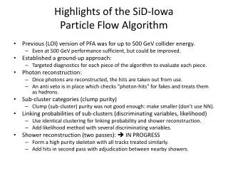
Basic Building Blocks of the (Iowa) PFA • MC hits within 100 ns from IP are digitized • Photon, Muon and Electron ID • Track and Seed Cluster (Directed Tree) • Building Charged Hadron Shower • Reconstructing Particles (four-vectors) Hits belonging to Photon, Muon and Electronare removed from the hit list for clustering algorithm Next Use DirectedTreeClustering for classifying the remaining hits into sub-cluster types like MIPs, Clumps, Blocks and `leftover’s Finally, start building Hadron Showers for one charged track at a time
Cluster Building • Extrapolate (each) track to the ECAL surface • Find Seed: sub-cluster directly connected to extrapolated track • Each track typically has one seed Special cases: track without seed, or does not reach calorimeter • Now start connecting other sub-clusters to the seed of each track • Start with lowest and then progressively higher momentum tracks • Up to ten iterations until all track-cluster match satisfy (E – p) within tolerance Connecting Clusters Scoring : (a poor man’s) Probability of a link Based on the sub-cluster type and geometric proximity a score between 0 and 1 is assigned between any two sub-clusters starting with the cluster in consideration The higher the score the higher the probability of a link A cut-off threshold is obtained for an energy by tuning with events
Energy dependence Performance at LOI Study just how much is contributed because of leakage
Leakage study at 500 GeV and 1 TeV • Produce data sets a SiD02-like detector MC with 6 HCAL for 1 TeV, 500 GeV, 200 GeV • Change Steel for Cu for absorber • Increase to 54 layers from 40 layers in HCAL • 1.7 more material in HCAL • No gap between HCAL and Muonendcap (instead of 10 cm) Compare sid02 with sid02-Cu at various energies Check leakage by observing # hits in Muon detector : punch thru; a measure of leakageSimultaneouslystudy the corresponding change in Energy resolutionThe relative measure from the two gives an approximate semi-quantitative measure of leakage vs performance Although substantial leakage is present at 500 GeV confusion is clearly important
Punch-through muon hits SiD02-Cu SiD02
Resolution study (SiD02-Cu comparison)real tracking SiD02-Cu SiD02
Conclusions from Leakage study • At 1 TeV leakage comparison shows large difference in performance between SiD-nominal (dashed) and SiD-Cu detectors (solid) • At 500 GeV leakage comparison shows significant difference in performance between SiD-nominal (dashed) and SiD-Cu detectors (solid) • Performance of 1 TeVSiD-Cu is similar to 500 GeVSiD-nominal in leakage • At 1 TeV performance in resolution is worse with SiD-nominal (dashed) and SiD-Cu detectors (solid) • At 500 GeV performance in resolution is worse with SiD-nominal (dashed) and SiD-Cu detectors (solid) • However : The difference of performance in resolution between 1 TeVSiD-Cu and 500 GeVSiD-nominal is not similar to that in leakage Although substantial leakage is present at 500 GeV, algorithm (confusion) has an important part
A 500 GeVqqbar event from one side jet Raw MC hits are displayed, each color shows an individual shower Contains a low energy 12 GeV neutral hadron and several photons in the ECAL; charged hadrons interacts
reconstructed The same as before shown without the isolated and unmatched hits : still no PFA reconstruction, only with knowledge of MC Now shown without the isolated hits but after reconstruction, alogorithm of charged hadron track-cluster match (cone algorithm) p (orange) = 119 GeV, E/p match, enough hits (green) = 17 GeV , algorithm introduced a cone-like path in the reclustering to pick up secondary neutrals; but ended up being too aggressive in stealing pieces from the low momenta tracks
has a low energy 12 GeV neutral hadron and several photons present in the ECAL; interaction of charged hadron p (orange) = 119 GeV, E/p match, enough hits (green) = 17 GeV reconstructed RefinedCheatCluster Diagnosis of `A’ problem: an example RefinedCluster - sharedhits Had introduced a cone-like path in the reclustering to pick up secondary neutrals; but ends up being too aggressive
The `Cone’ Algorithm Cluster DirAngle DCA Seed IP PosAngle Interaction point
All plots show variables defined for links between a seed and a cluster. If the seed and the cluster belong to the same truth particle, the link is quoted as “Signal” otherwise it is quoted as “Background” • Top-Left Plot:Scores just before the First cone algorithm runs. • Top-Middle Plot:Scores just after the First cone algorithm runs. • Top-Right Plot: Impact Parameter (IP): Distance between the center of the seed and the straight line from the center of the cluster extrapolated along the cluster’s direction • Bottom-Left Plot: Distance of closest approach (DCA) between two straight lines taken respectively from the center of the seed and the center of the cluster and along the respective directions. • Bottom-Middle Plot:Angle at the interaction point formed by the positions of the seed and the cluster. • Bottom-Right Plot:Angular difference between the direction of the seed and the direction of the cluster.
Score disteribution for links when the first cone algorithm modifiesthe score. • Left plot: • Scores before the first cone algorithm. • Right plot: • Scores after the cone algorithm. • While Signal/Background discrimination is better after the first cone algorithm, backgrounds now peak in the Signal region.
Correlated Variables now zoom on signal region: look at links when the first cone algorithm gives a high score (>0.8).
Sharing of hits: Breaking up into smaller clusters Extending to smaller pieces
Next Steps Allow flexibility in assignment of hits in clusters from tracks in the vicinity; Allocate after arbitration Check where exactly the `cone’ is needed, modify this, dump the rest Wait for results from ongoing study here…. Faster turn around time Improved resolution Next major step : Incorporate the PFA with realistic SiD (SiD03) geometry Now progressing in parallel Expect to take a step backward: non-trivial Improve sophisticated modifications for special types of clusters, like backscattering, complex rare occurrences
Particle Flow • Energy of a hadronic jet in a calorimeter Ejet = E (+0) + Ehadronic (neglecting ’s and leakage etc) Electromagnetic and hadronic components have different responsesSolutions: compensating calorimetry, measure hadronic and EM separately….. • However: Ejet = Ephotons+ Eneutral-hadrons + Echarged-hadrons Obtain Charged hadron energy (60) from trackingObtain photon/EM energy (30) from ECAL with 19/E resolution Get neutral hadron energy (10) from E/HCAL with 67/E resolution • Therefore the jet energy resolution is Ejet Echarged Ephotons Eneutral hadrons 0 19/(0.3 x Ejet) 67/(0.1 x Ejet) 20/E fantastic !
Particle Flow contd • The concept depends on ability to measure particles independently • Charged and neutral particle confusion degrades resolution Ejet Ephotons Eneutral hadrons confusion The confusion should be minimized in a good PFA Need excellent pattern recognition (also high granularity and low occupancy) • sid02 : ECAL: 30+1 layers of (320μm Si + 2.5/5.0mm W), 3.5 x 3.5mm cells. HCAL: 40 layers of (1.2mm RPC + 2cm steel), 1cm x 1cm cells.