Download
1 / 26
270 likes | 622 Vues
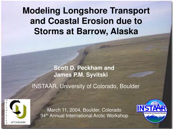
Modeling Longshore Transport and Coastal Erosion due to Storms at Barrow, Alaska. Scott D. Peckham and James P.M. Syvitski. INSTAAR, University of Colorado, Boulder. March 11, 2004, Boulder, Colorado 34 th Annual International Arctic Workshop.

E N D
Modeling Longshore Transport and Coastal Erosion due to Storms at Barrow, Alaska Scott D. Peckham and James P.M. Syvitski INSTAAR, University of Colorado, Boulder March 11, 2004, Boulder, Colorado 34th Annual International Arctic Workshop
This coastal erosion modeling project is part of a larger NSF Arctic System Science (ARCSS) Program project entitled: An Integrated Assessment of the Impacts of Climate Variability on the Alaskan North Slope Coastal Region Principal Investigators: Amanda Lynch, Ronald Brunner, Judith Curry, James Maslanik, Linda Mearns, Anne Jensen, Glenn Sheehan and James Syvitski It is also part of HARC: Human Dimensions of the Arctic
Geography Near Barrow, Alaska storm wind
Characteristics of Ocean Waves Wave number L = wavelength (m) Wave frequency T = wave period (s) Dispersion relation, Airy waves shallow ( d < 0.07 L ) Phase velocity or celerity deep ( d > 0.28 L ) Group velocity
Wave Refraction due to Shoaling Snell’s Law Approximation where Solve for wave angle where fis the contour angle. Wave vector angle
Wave Heights and Wave Breaking Wave height Refraction effect Shoaling effect Breaking wave conditions US Army Corps of Engineers Komar & Gaughan (1972) LeMehaute (1962) Miche criterion Deep water
Nearshore Sediment Transport Semi-empirical wave power formulation (Komar and Inman, 1970) Each variable on right-hand side is evaluated at the breaker zone. Longshore wave power Immersed-weight transport rate ( K = 0.7 for sand and K is unitless ) Volumetric transport rate (m3 / sec) ( a’ = (1 - p), usually taken as 0.6 ) Bed erosion and deposition Different grain sizes
Waves on a Fully-Developed Sea Fetch (miles) required to reach fully-developed sea state vs. wind speed (mph) Duration (hours) required to reach fully-developed sea state vs. wind speed (mph) Wave characteristics for peak frequency of fully developed sea ( ft ) ( sec ) Theoretical wave spectrum for a fully-developed sea ( ft )
Large Storms at Barrow, Alaska August 2000 Storm October 1963 Storm Winds from west Fetch of 500 miles 9 continuous hours over 35 mph 16 continuous hours over 30 mph Winds from west Fetch of 360 miles 14 continuous hours over 35 mph 18 continuous hours over 30 mph Fully-Developed Sea for 30 mph Wind Required Fetch = 212.4 miles Required Duration = 17.07 hours For both storms, fetch and duration are sufficient for FDS. Fully-Developed Sea for 35 mph Wind Required Fetch = 342.6 miles Required Duration = 23.6 hours For both storms, fetch is sufficient for FDS, but duration is too short. For a fully-developed sea in equilibrium with 30 mph wind, the dominant deep-water wave characteristics are predicted by theory to be: H = 9.6 feet, L = 189 feet, T = 7.4 seconds
Recasting the Longshore TransportEquation in Terms of FDS Values Volumetric transport rate ( m3 / s ) Longshore wave power Snell’s law Wave speed, shallow deep Breaking wave height in terms of FDS values Combining these equations with those that give H, L and T in terms of wind speed, w, for a fully-developed sea, we can write Q as: ( m3 / sec ) To change units to ( m3 / hour ), multiply Q by 3600. To change units to ( yard3 / hour ), multiply Q by 1.308.
Predicted Longshore TransportRate for Storms at Barrow, AK For Barrow’s coastline, with a sustained wind from due west, we have degrees, with a value of about 39 degrees at Barrow. Beach material is black, pea-sized gravel (0.5 to 1 cm), so we will use K = 0.45, rs = 3000 kg / m3, and a’ = 0.6 as initial estimates. For a fully-developed sea with a wind speed of 30 mph, we get: Q = 3934 (m3 / hour) or Q = 5145 (yd3 / hour) as the estimated sediment transport rate during both the August 2000 and October 1963 storms. For FDS conditions and a wind speed of 35 mph, we would get: Q = 10,230 (m3 / hour) or Q = 13,381 (yd3 / hour)
Simplified Coastal Erosion Model y = coastline position measured from a meridian line x = distance along this meridian line t = time d = closure depth Q = longshore sediment transport rate a = incoming wave angle Note that coastal erosion is predicted to be zero at points where Q reaches a maximum with respect to alpha (45 degrees) (as near Barrow) and for straight coastlines (via last term).
Conclusions The physical cause of longshore currents due to waves is well-understood and is well-described by mathematical models. Sediment transport due to longshore currents is less well understood, but can be described by an empirically validated formula due to Komar. This formula predicts maximum sediment transport for a breaking wave angle of 45 degrees, which is close to the value near Barrow, Alaska. A “nodal point” is predicted to occur near the city of Barrow, Alaska with erosion south of this point and deposition north of this point. This agrees with an analysis of remotely-sensed images. Longshore transport is a highly nonlinear function of sustained wind speed, so that relatively small changes in wind speed result in very large changes in sediment transport rates. The results presented here provide a practical method for residents of Barrow, Alaska to assess risk using real-time wind data and to understand why erosion or accretion occurs at particular locations along the coast.
References Dean, R.G. and Dalrymple, R.A. (19??) Coastal Processes: with Engineering Applications, Cambridge University Press. Ebersole, B.A. and Dalrymple, R.A. (1979) A numerical model for nearshore circulation including convective accelerations and lateral mixing, Technical Report No. 4, Contract No. N0014-76-C-0342, with ONR Research Geography Programs, Ocean Engineering Report No. 21, Dept. of Civil Engineering, Univ. of Delaware, Newark. Komar, P.D. (1998) Beach Processes and Sedimentation, 2nd ed., Prentice-Hall Inc., New Jersey, 544 pp. Lighthill, J. (1978) Waves in Fluids, Cambridge University Press, 504 pp. Longuet-Higgins, M.S. (1970) Longshore currents generated by obliquely incident sea waves, J. Geophysical Research, 75, 6778-6789. Longuet-Higgins, M.S. and Stewart, R.W. (19 64) Radiation stress in water waves: A physical discussion with application, Deep Sea Research, 11, 529-563. Martinez, P.A. and Harbaugh, J.W. (1993) Simulating Nearshore Environments, Pergamon Press, New York. U.S. Army Corps of Engineers (1984) Shore Protection Manual, Vol. 1, Coastal Engineering Research Center, Vicksburg, Mississippi.
Conclusions The physical cause of longshore currents due to waves is well-understood and is well-described by mathematical models. The following physical effects can all be captured by this model: (1) conservation of mass and momentum (and energy) (2) refraction of waves due to shoaling (3) the effects of waves interacting with mean currents (4) the effect of breaking waves in the surf zone (5) lateral mixing across the breaker zone due to turbulence (6) wave set-up and set-down (surface displacement) (7) rip currents and vortices Sediment transport due to longshore currents is less well understood, but can be described by an empirically validated formula due to Komar. This last part of the model is not yet fully implemented. Further work is need to fully understand the nature of numerical instabilities in the model and the approach to steady state.
Derivation of Wave Height Equation Figure 5-42 from Komar (1976) Straight beach with parallel contour lines
Mass and Momentum Conservation Equations of motion are depth-integrated and time-averaged over one wave period. These can be iterated until steady-state conditions are achieved. Wave set-up and set-down
Radiation Stress Terms Radiation stress includes excess momentum flux and pressure terms due to waves. Original formulation due to Longuet-Higgins (1962). Where q is the wave angle, E is the energy density of the wave per unit area, H is the wave height, d is the water depth, k is the wave number and Cg is the group velocity.
Frictional Loss via Bed Stress Bed stress has a quadratic dependence on the total velocity, which is composed of mean currents (U, V) and orbital velocities due to waves (u cos(q), v cos(q)). Shear stress on the bed where the total velocity is given by Wave orbital velocity Max orbital velocity
Equations that Govern Waves Wave number vector field k is irrotational ( This implies that k = grad(f). ) Dispersion relation between frequency and wave number Solution via Newton iteration Wave-current interaction equation