Download
1 / 17
180 likes | 543 Vues
Solving Linear Programming Problems Shubhagata Roy.

E N D
Q. What is a Linear Programming Problem?A. A Linear Programming Problem(LPP) is a problem in which we are asked to find the maximum (or minimum) value of a linear objective functionZ = aX1 + bX2 + cX2 + ... (e.g. Z = 3X1 + 2X2 + X3)Subject to one or more linear constraints of the formAX1+ BX2 + CX3 + . . <or= N (e.g. X1 + X2 + 3X3 <or= 12)The desired largest (or smallest) value of the objective function is called the optimal value, and a collection of values of X1,X2,X3, . . . that gives the optimal value constitutes an optimal solution.The variables X1, X2, X3, . . are called the decision variables.
Simplex MethodThe most frequently used method to solve LP problems is the Simplex Method. Before going into the method, we must get familiarized with some important terminologies :Standard Form- A linear program in which all the constraints are written as equalities.Slack Variable- A variable added to the LHS of “Less than orequal to” constraint to convert it into an equality.Surplus Variable- A variable subtracted from the LHS of “More than orequal to” constraint to convert it into an equality.Basic Solution- For a system of m linear equations in n variables (n>m),a solution obtained by setting (n-m) variables equal to zeroand solving the system of equations forremaining m variables.Basic Feasible Solution(BFS)- If all the variables in basic solution are more than or equal to zero.
Optimum Solution-Any BFS which optimizes(maximizes or minimizes) the objective function.Tableau Form- When a LPP is written in a tabular form prior to setting up the Initial Simplex Tableau.Simplex Tableau- A table which is used to keep track of the calculations made at each iteration when the simplex method is employed.Net EvaluationRow(Cj-Zj )- The row containing net profit or loss.The nos.in this row are also known as shadow prices.Pivotal Column- The column having largest positive(or negative) value in the Net Evaluation Row for a maximization(or minimization) problem.Pivotal Row- The row corresponding to variable that will leave the table in order to make room for another variable.Pivotal Element- Element at the intersection of pivotal row and pivotal column.
To understand the method,let us take an example containing two decision variables and two constraints.Example:Maximize Z = 7X1+5X2 , subject to the constraints, X1+2X2 < or = 6 4X1+3X2 < or = 12 and X1 & X2are non-negative.Step1: Convert the LP problem into a system of linear equations.We do this by rewriting the constraint inequalities as equations by adding new "slack variables" and assigning them zero coefficients(profits) in the objective function as shown below: X1+2X2+S1 = 6 4X1+3X2 +S2 = 12And the Objective Function would be:Z=7X1+5X2+0.S1+0.S2
Step 2: Obtain a Basic Solution to the problem.We do this by putting the decision variables X1=X2=0,so that S1= 6 and S2=12.These are the initial values of slack variables.Step 3: Form the Initial Tableau as shown.
Step 4: Find (Cj-Zj) having highest positive value.The column corresponding to this value,is called the Pivotal Column and enters the table. In the previous table,column corresponding to variable X1 is the pivotal column.Step 5: Find the Minimum Positive Ratio.Divide XB values by the corresponding values of Pivotal Column.The row corresponding to the minimum positive value is the Pivotal Row and leaves the table. In the previous table,row corresponding to the slack variable S2 is the pivotal row.
Step 6: First Iteration or First Simplex Tableau.In the new table,we shall place the incoming variable(X1) instead of the outgoing variable(S2). Accordingly,new values of this row have to be obtained in the following way :R2(New)=R2(Old)/Pivotal Element = R2(Old)/4R1(New)=R1(Old) - (Intersecting value of R1(Old) & Pivotal Col)*R2(New) =R1(Old) - 1*R2(New)
Step 7: If all the (Cj-Zj) values are zero or negative,an optimum point is reached otherwise repeat the process as given in Step 4,5 & 6.Since all the (Cj-Zj) values are either negative or zero,hence an optimum solution has been achieved.The optimum values are:X1=3,X2=0 and,Max Z=21.
Big-M Method of solving LPP The Big-M method of handling instances with artificial variables is the “commonsense approach”. Essentially, the notion is to make the artificial variables, through their coefficients in the objective function, so costly or unprofitable that any feasible solution to the real problem would be preferred....unless the original instance possessed no feasible solutions at all. But this means that we need to assign, in the objective function, coefficients to the artificial variables that are either very small (maximization problem) or very large (minimization problem); whatever this value,let us call it Big M. In fact, this notion is an old trick in optimization in general; we simply associate a penalty value with variables that we do not want to be part of an ultimate solution(unless such an outcome Is unavoidable).
Indeed, the penalty is so costly that unless any of the respective variables' inclusion is warranted algorithmically,such variables will never be part of any feasible solution.This method removes artificial variables from the basis. Here, we assign a large undesirable (unacceptable penalty) coefficients to artificial variables from the objective function point of view. If the objective function (Z) is to be minimized, then a very large positive price (penalty, M) is assigned to each artificial variable and if Z is to be minimized, then a very large negative price is to be assigned. The penalty will be designated by +M for minimization problem and by –M for a maximization problem and also M>0.
Example: Minimize Z= 600X1+500X2subject to constraints,2X1+ X2 >or= 80 X1+2X2 >or= 60 and X1,X2 >or= 0Step1: Convert the LP problem into a system of linear equations.We do this by rewriting the constraint inequalities as equations by subtracting new “surplus & artificial variables" and assigning them zero & +M coefficientsrespectively in the objective function as shown below.So the Objective Function would be: Z=600X1+500X2+0.S1+0.S2+MA1+MA2subject to constraints,2X1+ X2-S1+A1 = 80 X1+2X2-S2+A2 = 60X1,X2,S1,S2,A1,A2 >or= 0
Step 2: Obtain a Basic Solution to the problem.We do this by putting the decision variables X1=X2=S1=S2=0,so that A1= 80 and A2=60. These are the initial values of artificial variables.Step 3: Form the Initial Tableau as shown.
It is clear from the tableau that X2 will enter and A2 will leave the basis. Hence 2 is the key element in pivotal column. Now,the new row operations are as follows:R2(New) = R2(Old)/2R1(New) = R1(Old) - 1*R2(New)
It is clear from the tableau that X1 will enter and A1 will leave the basis. Hence 2 is the key element in pivotal column. Now,the new row operations are as follows:R1(New) = R1(Old)*2/3R2(New) = R2(Old) – (1/2)*R1(New)
Since all the values of (Cj-Zj)are either zero or positive and also both the artificial variables have been removed, an optimum solution has been arrived at with X1=100/3 , X2=40/3 and Z=80,000/3.