Download
1 / 51
510 likes | 634 Vues
ECE 598: The Speech Chain. Lecture 12: Information Theory. Today. Information Speech as Communication Shannon’s Measurement of Information Entropy Entropy = Average Information “Complexity” or “sophistication” of a text Conditional Entropy

E N D
ECE 598: The Speech Chain Lecture 12: Information Theory
Today • Information • Speech as Communication • Shannon’s Measurement of Information • Entropy • Entropy = Average Information • “Complexity” or “sophistication” of a text • Conditional Entropy • Conditional Entropy = Average Conditional Information • Example: Confusion Matrix, Articulation Testing • Conditional Entropy vs. SNR • Channel Capacity • Mutual Information = Entropy – Conditional Entropy • Channel Capacity = max{Mutual Information} • Finite State Language Models • Grammars • Regular Grammar = Finite State Grammar = Markov Grammar • Entropy of a Finite State Grammar • N-Gram Language Models • Maximum-Likelihood Estimation • Cross-Entropy of Text given its N-Gram
Speech as Communication I said these words: […,wn,…] Acoustic Noise, Babble, Reverberation, … I heard these words: […,ŵn,…] • wn, ŵn = words selected from vocabulary V • Size of the vocabulary, |V|, is assumed to be finite. • No human language has a truly finite vocabulary!!! • For a more accurate analysis, we should do a phoneme-by-phoneme analysis, i.e., wn, ŵn= phonemes in language V • If |V| is finite, then we can define p(wn|hn): • hn = all relevant history, including • previous words of the same utterance, w1,…,wn-1 • Dialog history (what did the other talker just say?) • Shared knowledge, e.g., physical knowledge, cultural knowledge • 0 ≤ p(wn|hn) ≤ 1 • Swn in V p(wn|hn) = 1 + Noisy Speech Speech (Acoustic Signal)
Shannon’s Criteria for a Measure of “Information” Information should be… • Non-negative • I(wn|hn) ≥ 0 • Zero if a word is perfectly predictable from its history • I(wn|hn) = 0 if and only if p(wn|hn) = 1 • Large for unexpected words • I(wn|hn) is large if p(wn|hn) is small • Additive • I(wn-1,wn) = I(wn-1) + I(wn)
Shannon’s Measure of Information All of the criteria are satisfied by the following definition of information: I(wn) = loga(1/p(wn|hn)) = -loga p(wn|hn)
Information Information is… • Non-negative: p(wn|hn)<1 logap(wn|hn)<0 I(wn|hn)>0 • Zero if a word is perfectly predictable: p(wn|hn)=1 logap(wn|hn)=0 I(wn|hn)=0 • Large if a word is unpredictable: I(wn)= -logap(wn|hn) large if p(wn|hn) small • Additive: p(wn-1,wn) = p(wn-1)p(wn) -logap(wn-1,wn) = -logap(wn-1) -logap(wn) I(wn-1,wn) = I(wn-1) + I(wn)
Bits, Nats, and Digits • Consider a string of random coin tosses, “HTHHHTTHTHHTTT” • p(wn|hn) = ½ • -log2 p(wn|hn) = 1 bit of information/symbol • -ln p(wn|hn) = 0.69 nats/bit • -log10 p(wn|hn) = 0.3 digits/bit • Consider a random string of digits, “49873417” • p(wn|hn) = 1/10 • -log10 p(wn|hn) = 1 digit/symbol • -log2 p(wn|hn) = 3.32 bits/digit • -ln p(wn|hn) = 2.3 nats/digit • Unless otherwise specified, information is usually measured in bits I(w|h) = -log2 p(w|h)
Entropy = Average Information • How unpredictable is the next word? • Entropy = Average Unpredictability H(p) = Sw p(w) I(w) H(p) = -Sw p(w) log2p(w) • Notice that entropy is not a function of the word, w… • It is a function of the probability distribution, p(w)
Example: Uniform Source • Entropy of a coin toss: H(p) = -p(“heads”)log2p(“heads”)-p(“tails”)log2p(“tails”) =-0.5 log2(0.5)-0.5 log2(0.5) = 1 bit/symbol • Entropy of uniform source with N different words: p(w) = 1/N H(p) = - Sw=1N p(w)log2p(w) = log2N • In general: if all words are equally likely, then the average unpredictability (“entropy”) is equal to the unpredictability of any particular word (the “information” conveyed by that word): log2N bits.
Example: Non-Uniform Source • Consider the toss of a weighted coin, with the following probabilities: p(“heads”) = 0.6 p(“tails”) = 0.4 • Information communicated by each word: I(“heads”) = -log2 0.6 = 0.74 bits I(“tails”) = -log2 0.4 = 1.3 bits • Entropy = average information H(p) = -0.6 log2(0.6)-0.4 log2(0.4) = 0.97 bits/symbol on average • The entropy of a non-uniform source is always less than the entropy of a uniform source with the same vocabulary. • Entropy of a uniform source, N-word vocabulary, is log2N bits • Information conveyed by a likely word is less than log2N bits • Information conveyed by an unlikely word is more than log2N bits --- but that word is unlikely to occur!
Example: Deterministic Source • Consider the toss of a two-headed coin, with the following probabilities: p(“heads”) = 1.0 p(“tails”) = 0.0 • Information communicated by each word: I(“heads”) = -log2 1.0 = 0 bits I(“tails”) = -log2 0.0 = infinite bits!! • Entropy = average information H(p) = -1.0 log2(1.0)-0.0 log2(0.0) = 0 bits/symbol on average • If you know in advance what each word will be… • then you gain no information by listening to the message. • The “entropy” (average information per symbol) is zero.
Example: Textual Complexity Twas brillig, and the slithy toves did gyre and gimble in the wabe… • p(w) = 2/13 for w=“and,” w=“the” • p(w) = 1/13 for the other 9 words H(p) = -Swp(w)log2p(w) = -2(2/13)log2(2/13)-9(1/13)log2(1/13) = 3.4 bits/word
Example: Textual Complexity How much wood would a woodchuck chuck if a woodchuck could chuck wood? • p(w) = 2/13 for “wood, a, woodchuck, chuck” • p(w) = 1/13 for the other 5 words H(p) = -Swp(w)log2p(w) = -4(2/13)log2(2/13)-5(1/13)log2(1/13) = 3.0 bits/word
Example: The Speech Channel How much wood wood a wood chuck chuck if a wood chuck could chuck wood? • p(w) = 5/15 for w=“wood” • p(w) = 4/15 for w=“chuck” • p(w) = 2/15 for w=“a” • p(w) = 1/15 for “how, much, if, could” H(p) = -Swp(w)log2p(w) = 2.5 bits/word
Conditional Entropy = Average Conditional Information • Suppose that p(w|h) is “conditional” upon some history variable h. Then the information provided by w is I(w|h) = -log2 p(w|h) • Suppose that we also know the probability distribution of the history variable, p(h) • The joint probability of w and h is p(w,h) = p(w|h)p(h) • The average information provided by any word, w, averaged across all possible histories, is the “conditional entropy” H(p(w|h)): H(p(w|h)) = SwSh p(w,h) I(w|h) = -Sh p(h) Sw p(w|h) log2p(w|h)
Example: Communication I said these words: […,wn,…] Acoustic Noise, Babble, Reverberation, … I heard these words: […,ŵn,…] • Suppose w, ŵ are not always the same • … but we can estimate the probability p(ŵ|w) • Entropy of the source is H(p(w)) = -Sw p(w) log2p(w) • Conditional Entropy of the received information is H(p(ŵ|w)) = -Swp(w) Sŵ p(ŵ|w) log2p(ŵ|w) • Conditional Entropy of Received Message given the Transmitted Message is called Equivocation + Noisy Speech Speech (Acoustic Signal)
Example: Articulation Testing “a tug” “a sug” “a fug” Acoustic Noise, Babble, Reverberation, … “a tug” “a thug” “a fug” • The “caller” reads a list of nonsense syllables • Miller and Nicely, 1955: only one consonant per utterance is randomized • Fletcher: CVC syllables, all three phonemes are randomly selected • The “listener” writes down what she hears • The lists are compared to compute p(ŵ|w) + Noisy Speech Speech (Acoustic Signal)
Confusion Matrix: Consonants at -6dB SNR(Miller and Nicely, 1955) Perceived (ŵ) Called (w)
Conditional Probabilities p(ŵ|w), 1 signif. dig.(Miller and Nicely, 1955) Perceived (ŵ) Called (w)
Example: Articulation Testing, -6dB SNR • At -6dB SNR, p(ŵ|w) is nonzero for about 4 different possible responses • The equivocation is roughly H(p(ŵ|w)) = -Swp(w) Sŵ p(ŵ|w) log2p(ŵ|w) = -Sw (1/18) Sŵ (1/4) log2 (1/4) = -18(1/18)4(1/4)log2(1/4) = 2 bits
Example: Perfect Transmission • At very high signal to noise ratio (for humans, SNR > 18dB)… • The listener understands exactly what the talker said: • p(ŵ|w)=1 (for ŵ=w) or • p(ŵ|w)=0 (for ŵ≠w) • So H(p(ŵ|w))=0 --- zero equivocation • Meaning: If you know exactly what the talker said, then that’s what you’ll write; there is no more randomness left
Example: No Transmission • At very low signal to noise ratio (for humans, SNR < minus 18dB)… • The listener doesn’t understand anything the talker said: • p(ŵ|w)=p(ŵ) • The listener has no idea what the talker said, so she has to guess. • Her guesses follow the natural pattern of the language: she is more likely to write /s/ or /t/ instead of /q/ or /ð/. • So H(p(ŵ|w))=H(p(ŵ))=H(p(w)) --- conditional entropy is exactly the same as the original source entropy • Meaning: If you have no idea what the talker said, then you haven’t learned anything by listening
Equivocation as a Function of SNR Region 1: No Transmission; Random Guessing Equivocation = Entropy of the Language Dashed Line = Entropy of the Language (e.g., for 18-consonant articulation testing, source entropy H(p(w))=log218 bits) Equivocation (Bits) Region 2: Equivocation depends on SNR Region 3: Error-Free Transmission Equivocation = 0 -18dB 18dB SNR
Definition: Mutual Information • On average, how much information gets correctly transmitted from caller to listener? • “Mutual Information” = • Average Information in the Caller’s Message • …minus… • Conditional Randomness of the Listener’s Perception • I(p(ŵ,w)) = H(p(w)) – H(p(ŵ|w))
Listeners use Context to “Guess” the Message Consider gradually increasing the complexity of the message in a noisy environment • Caller says “yes, yes, no, yes, no.” Entropy of the message is 1 bit/word; listener gets enough from lip-reading to correctly guess every word. • Caller says “429986734.” Entropy of the message is 3.2 bits/word; listener can still understand just by lip reading. • Caller says “Let’s go scuba diving in Puerto Vallarta this January.” • Listener effortlessly understands the low-entropy parts of the message (“let’s go”), but • The high-entropy parts (“scuba diving,” “Puerto Vallarta”) are completely lost in the noise
The Mutual Information Ceiling Effect Region 2: Mutual Information clipped at an SNR-dependent maximum bit rate called the “channel capacity.” Equivocation = Source Entropy – Channel Capacity Region 1: Perfect Transmission Equivocation=0 Mutual Information= Source Entropy Mutual Information Transmitted (Bits) Equivocation (Bits) Source Message Entropy (Bits)
Definition: Channel Capacity • Capacity of a Channel = Maximum number of bits per second that may be transmitted, error-free, through that channel • C = maxp I(p(ŵ,w)) • The maximum is taken over all possible source distributions, i.e., over all possible H(p(w))
Information Theory Jargon Review • Information = Unpredictability of a word I(w) = -log2p(w) • Entropy = Average Information of the words in a message H(p(w)) = -Sw p(w) log2p(w) • Conditional Entropy = Average Conditional Information H(p(w|h)) = -Sh p(h) Sw p(w|h) log2p(w|h) • Equivocation = Conditional Entropy of the Received Message given the Transmitted Message H(p(ŵ|w)) = -Swp(w) Sŵ p(ŵ|w) log2p(ŵ|w) • Mutual Information = Entropy minus Equivocation I(p(ŵ,w)) = H(p(w)) – H(p(ŵ|w)) • Channel Capacity = Maximum Mutual Information C(SNR) = maxp I(p(ŵ,w))
Grammar • Discussion so far has ignored the “history,” hn. • How does hn affect p(wn|hn)? • Topics that we won’t discuss today, but that computational linguists are working on: • Dialog context • Shared knowledge • Topics that we will discuss: • Previous words in the same utterance: p(wn|w1,…,wn-1) ≠ p(wn) • A grammar = something that decides whether or not (w1,…,wN) is a possible sentence. • Probabilistic grammar = something that calculates p(w1,…,wN)
Grammar • Definition: A Grammar, G, has four parts G = { S, N, V, P } • N = A set of “non-terminal” nodes • Example: N = { Sentence, NP, VP, NOU, VER, DET, ADJ, ADV } • V = A set of “terminal” nodes, a.k.a. a “vocabulary” • Example: V = { how, much, wood, would, a } • S = The non-terminal node that sits at the top of every parse tree • Example: S = { Sentence } • P = A set of production rules • Example (CFG in “Chomsky normal form”): Sentence = NP VP NP = DET NP NP = ADJ NP NP = NOU NOU = wood NOU = woodchuck
Types of Grammar • A type 0 (“unrestricted”) grammar can have anything on either side of a production rule • A type 1 (“context sensitive grammar,” CSG) has rules of the following form: <context1> N <context2> = <context1> STUFF <context2> …where… • <context1> and <context2> are arbitrary unchanged contexts • N is an arbitrary non-terminal, e.g., “NP” • STUFF is an arbitrary sequence of terminals and non-terminals, e.g., “the big ADJ NP” would be an acceptable STUFF • A type 2 grammar (“context free grammar,” CFG) has rules of the following form: N = STUFF • A type 3 grammar (“regular grammar,” RG) has rules of the following form: N1 = T1 N2 • N1, N2 are non-terminals • T1 is a terminal node – a word! • Acceptable Example: NP = the NP • Unacceptable Example: Sentence = NP VP
Regular Grammar = Finite State Grammar (Markov Grammar) • Let every non-terminal be a “state” • Let every production rule be a “transition” • Example: • S = a S • S = woodchuck VP • VP = could VP • VP = chuck NP • NP = how QP • QP = much NP • NP = wood QP how could much a woodchuck chuck wood S VP NP END
Probabilistic Finite State Grammar • Every production rule has an associated conditional probability: p(production rule | LHS nonterminal) • Example: • S = a S 0.5 • S = woodchuck VP 0.5 • VP = could VP 0.7 • VP = chuck NP 0.3 • NP = how QP 0.4 • QP = much NP 1.0 • NP = wood 0.6 how (0.4) QP could (0.7) much (1.0) a (0.5) woodchuck (0.5) chuck (0.3) wood (0.6) S VP NP END
Calculating the probability of text how (0.4) QP could (0.7) • p(“a woodchuck could chuck how much wood”) = (0.5)(0.5)(0.7)(0.3)(0.4)(1.0)(0.6) = 0.0126 • p(“woodchuck chuck wood”) = (0.5)(0.3)(0.6) = 0.09 • p(“A woodchuck could chuck how much wood. Woodchuck chuck wood.”) = (0.0126)(0.09) = 0.01134 • p(some very long text corpus) = p(1st sentence)p(2nd sentence)… much (1.0) a (0.5) woodchuck (0.5) chuck (0.3) wood (0.6) S VP NP END
Cross-Entropy • Cross-entropy of an N-word text, T, given a language model, G: H(T|G) = -Sn=1N p(wn|T) log2p(wn|G,hn) = -Sn=1N (1/N) log2p(wn|G,hn) • N = # words in the text • p(wn|T) = (# times wn occurs)/N • p(wn|G) = probability of word wn given its history hn, according to language model G
Cross-Entropy: Example how (0.4) QP could (0.7) • T = “A woodchuck could chuck wood.” • H(T|G) = = -Sn=1N p(wn|T) log2p(wn|G,hn) = -(1/N) Sn=1N log2p(wn|G,hn) = -(1/5) { log2(0.5) + log2(0.5) + log2(0.7)+ log2(0.3)+ log2(0.6) } = 4.989/5 = 0.998 bits • Interpretation: language model G assigns entropy of 0.998 bits to the words in text T. • This is a very low cross-entropy: G predicts T very well. much (1.0) a (0.5) woodchuck (0.5) chuck (0.3) wood (0.6) S VP NP END
N-Gram Language Models • An N-gram is just a PFSG (probabilistic finite state grammar) in which each nonterminal is specified by the N-1 most recent terminals. • Definition of an N-gram: p(wn|hn) = p(wn|wn-N+1,…,wn-1) • The most common choices for N are 0,1,2,3: • Trigram (3-gram): p(wn|hn) = p(wn|wn-2,wn-1) • Bigram (2-gram): p(wn|hn) = p(wn|wn-1) • Unigram (1-gram): p(wn|hn) = p(wn) • 0-gram: p(wn|hn) = 1/|V|
Example: A Woodchuck Bigram • T = “How much wood would a woodchuck chuck if a woodchuck could chuck wood” • Nonterminals are labeled by wn-1. Edges are labeled with wn, and with p(wn|wn-1) wood (0.5) could (0.5) how (1.0) much (1.0) wood (1.0) if (0.5) a (1.0) woodchuck (1.0) 0 how much wood would a woodchuck chuck if could chuck (0.5) would (1.0) chuck (1.0) a (1.0)
N-Gram: Maximum Likelihood Estimation • An N-gram is defined by its vocabulary V, and by the probabilities P = { p(wn|wn-N+1,…,wn-1) } G = { V, P } • A text is a (long) string of words, T = { w1,…,wN } • The probability of a text given an N-gram is p(T|G) = -Sn=1N p(wn|T) log2p(wn|G, wn-N+1,…,wn-1) = - (1/N) Sn=1N log2p(wn|G, wn-N+1,…,wn-1) • The “Maximum Likelihood” N-gram model is the set of probabilities, P, that maximizes p(T|G).
N-Gram: Maximum Likelihood Estimation • The “Maximum Likelihood” N-gram model is the set of probabilities, P, that maximizes p(T|G). These probabilities are given by: p(wn|wn-N+1,…,wn) = N(wn-N+1,…,wn)/N(wn-N+1,…,wn-1) • where • N(wn-N+1,…,wn) is the “frequency” of the N-gram wn-N+1,…,wn (i.e., the number of times that the N-gram occurs in the data) • N(wn-N+1,…,wn-1) is the frequency of the (N-1)-gram wn-N+1,…,wn-1 • This is the set of probabilities you would have guessed, anyway!! • For example, the woodchuck bigram assigned p(wn|wn-1)=N(wn-1,wn)/N(wn).
Cross-Entropy of an N-gram • Cross-entropy of an N-word text, T, given an N-gram G: H(T|G) = -Sn=1N p(wn|T) log2p(wn|G,wn-N+1,…,wn-1) = - (1/N) Sn=1N log2p(wn|G,wn-N+1,…,wn-1) • N = # words in the text • p(wn|T) = (# times wn occurs)/N • p(wn|G, wn-N+1,…,wn-1) = probability of word wn given its history wn-N+1,…,wn-1, according to N-gram language model G
Example: A Woodchuck Bigram • T = “a woodchuck could chuck wood.” • H(T|G) = -(1/5){log2(p(“a”))+log2(1.0)+log2(0.5)+log2(1.0)+log2(0.5)} = (2-log2p(“a”))/5 = 0.4 bits/word plus the information of the first word wood (0.5) could (0.5) much (1.0) wood (1.0) if (0.5) a (1.0) woodchuck (1.0) how much wood would a woodchuck chuck if could chuck (0.5) would (1.0) chuck (1.0) a (1.0)
Example: A Woodchuck Bigram • Information of the first word must be set by assumption. Common assumptions include: • Assume that the first word gives zero information (p(“a”)=1, log2(p(“a”))=0) --- this focuses attention on the bigram • First word information given by its unigram probability (p(“a”)=2/13, log2(p(“a”))=2.7 bits) --- this gives a well-normalized entropy • First word information given by its 0-gram probability (p(“a”)=1/9, log2(p(“a”))=3.2 bits) --- a different well-normalized entropy wood (0.5) could (0.5) much (1.0) wood (1.0) if (0.5) a (1.0) woodchuck (1.0) how much wood would a woodchuck chuck if could chuck (0.5) would (1.0) chuck (1.0) a (1.0)
N-Gram: Review • The “Maximum Likelihood” N-gram model is the set of probabilities, P, that maximizes p(T|G). These probabilities are given by: p(wn|wn-N+1,…,wn) = N(wn-N+1,…,wn)/N(wn-N+1,…,wn-1) • where • N(wn-N+1,…,wn) is the “frequency” of the N-gram wn-N+1,…,wn (i.e., the number of times that the N-gram occurs in the data) • N(wn-N+1,…,wn-1) is the frequency of the (N-1)-gram wn-N+1,…,wn-1 • This is the set of probabilities you would have guessed, anyway!! • For example, the woodchuck bigram assigned p(wn|wn-1)=N(wn-1,wn)/N(wn).