Topic 1- Statistical Analysis

1. Topic 1- Statistical Analysis

2. Why? • The scientific method involves making observations and collecting measurable data. • When measuring data from a sample, the sample must be representative of the entire population of that sample • Statistics allows us to sample small populations and draw conclusions of the larger populations

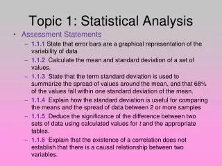
3. Why? • It allows us to measure differences and relationships between sets of data. • All conclusions drawn from an experiment have a certain level of confidence, but nothing in science is 100% certain.

4. What is a representative sample? • A small group whose characteristics accurately reflect those of the larger population from which it is drawn. • A representative sample is needed in order to make more accurate generalizations of the larger population • Example: If approximately 15% of the United States’ population is of Hispanic descent, a sample of 100 Americans also ought to include around 15 Hispanic people to be representative.

5. How do we get a representative sample? • Avoiding selection bias- when sampling is not representative as a result of convenience sampling (using just mpsj students) , undercoverage (not targeting a specific group of a population), judgement sampling (targeting individuals you pre-assume to fit a criteria) and non-response (people choose not to complete the experiment) • Larger sample sizes- ensures the sample is more similar to the original population • Random Sampling- selecting individuals from random areas ,times or with different methods • This results in better data collection quality and experimenter bias or placebo effect

6. Reliable and valid data • reliabilityis used to describe the overall consistency of a measure. A measure is said to have a high reliability if it produces similar results under consistent conditions. For example, measurements of people’s height and weight are often extremely reliable. • validityis the extent to which a concept,conclusion or measurement is well-founded and corresponds accurately to the real world. “You are measuring what you’re supposed to measure”

7. Range • Measures the spread of data • The difference between the largest and smallest observed values • If one data point is unusually large/small, it has a great effect on the range and is called an outlier (Outliers can often indicate an error in the experiment and are often eliminated).

8. Averages • Averages are the central tendencies of the data. There are three types; • Mean- sum of all the results divided by the number of results • Median- the middle value of a range of results • Mode: the value that appears the greatest number of times

9. Example • Find the mean, median and mode of the following data set • 1, 2, 2, 5, 6, 7, 11, 11, 11, 12 • Mean- = 6.8 • Median- = 6.5 • Mode-11 • When no numbers repeat then you do not have a mode • If the mean, median and mode are all approximately the same then we can assume a normal distribution

10. Averages • Averages do not tell us everything about a sample. • May not be representative of the entire population • Two samples of a populations could be different from one another. Bound to have natural variation

11. Standard Deviation • Samples can be very uniform- bunched around the mean or spread out a long way from the mean • The statistic that measures this spread is called the standard deviation

12. Standard deviation • A measure of how the individual data points are distributed around the mean • Allows us to compare the means\spread of data between two or more samples • Tells us how tightly the data points are clustered around the mean and therefore how many outliers there are in the data. • When the data points are clustered, the SD is very small and when spread apart the SD is large

13. Standard deviation and error bars • A graphical representation of variability • Can be used to show range of data or SD • In design labs, students often use their SD to represent their error bars on their graphs • A large SD indicates large error or non-valid results

14. Example • Calculate the SD of a sample- Four children are aged 5; 6; 8 and 9. • Step 1: find the mean  x= • x1= 5, x2=6, x3=8, x4=9 and N(population =4) • x= (x1 + x2 + x3 + x4) • x=7

15. Step 2 Find the SD σ: • σ = • σ= • σ = (5-7)2 + (6-7)2 + (8-7)2 + (9-7)2 • σ= 1.58 • Therefore the average age of the children is 7

16. Distribution • Consider a population of bean plants with a mean height of 7cm • Normal Distribution- A spread of data that is equally distributed before and after the mean • A flat bell curve- data widely spread • A tall and narrow curve- data is very close to the mean • Standard normal curve- 68% of all values lie within +/- 1 SD from the mean and 95% of all values lie within +/- 2 SD from the mean • As the distribution of a bell curve changes the SD value will change to account for the 68% and 95% of the data set.

17. = 68% or +/- 1

18. The t-test • To assess whether the means of two groups are statistically different from each other • Used when you want to compare the means of two groups • Ex. Is there a statistical difference in the mean height between a group of boys and girls at the age of 12?

19. The t-test • Notice that all three examples below have the same difference between means • Yet they all tell different stories. They all have different variability. • The two groups with low variability from their mean are visibly most different from each other and the groups with high variability are most similar to each other

20. T-test • We can judge the difference between means relative to their spread or variability using the t-test • The formula is a ratio;

21. The formula

22. Example • Problem:Sam Sleepresearcher hypothesizes that people who are allowed to sleep for only four hours will score significantly lower than people who are allowed to sleep for eight hours on a cognitive skills test. He brings 8participants into his sleep lab and randomly assigns them to one of two groups. In one group he has participants sleep for eight hours and in the other group he has them sleep for four. The morning after he administers the SCAT (Sam's Cognitive Ability Test) to the participants. (Scores on the SCAT range from 1-9 with high scores representing better performance).

23. Step 1- calculate degree of freedom Df (paired t-test)= sample size-1 Df (unpaired) = n1+n2 - 2

24. Step 1: Find the means for both groups and subtract Step 2: Calculate the variance (SD2) Step 3: Divide each variance by the sample size Step 4: Square root the denominator Mx8hours= 5 My4hours= 4 SD8=4.571 SD4=6.571 N8hours=8 and n4=8

25. Step 3- use t-table • Once the t-value is calculated you look it up in a table of significance to see whether the ratio (t-value) is large enough to say that the difference between the groups is not likely due to chance • Statisticians like to be 95% confident that their conclusions are significant. So we use the risk value or pvalue of p<0.05. Differences are due to chance 5% of the time vs. p=0.1 where error occurs 10% of the time • If p>0.05, this indicates the means are not statistically different

27. according to the t sig/probability table with df=n-1= 7, t must be at least 1.895to be significant • since our t=0.847 and therefore p>0.05, (it would fall at a lower confidence level between .25 and .1) this difference is not statistically significant

28. Correlation vs. Causation • “correlation does not imply causation”- means that correlation cannot be used to infer a causal relationships, but rather that the causes underlying the correlation may be indirect or unknown • Cause: a carefully designed experiment and its evidence can determine that A causes B • Correlation: observations, without a controlled experiment, can only show that A and B are related

29. Fallacy Examples • Ice cream sales correlate with the number of people who drown at sea. Therefore ice cream causes people to drown. • Children who sleep with a light on are more likely to develop myopia (nearsightedness) • Does light cause myopia? • Atmospheric CO2 has been climbing in conjunction with increased crime • Does CO2 cause crime?

30. A mathematical correlation test produces a value r, which signifies the correlation between two events • r+1 positive correlation (as X increases so does Y) • r =0 no correlation • r -1 negative correlation (as X increases Y decreases)

31. Accuracy & Precision • Accuracy: how close a measured value is to the true value • Precision: how close the measured values are to each other

32. Errors and Uncertainties • Examples: • Human errors- can occur when tools or instruments are used or read incorrectly. (E.g a thermometer reading must be taken after stirring and the bulb still in the liquid but not touching the bottom) • Systematic- experimenter does not know how to use the equipment or something wrong with equipment. • Random – unknown or unpredictable changes

33. Systematic • Note that systematic and random errors refer to problems associated with making measurements. Mistakes made in the calculations or in reading the instrument are not considered in error analysis. It is assumed that the experimenters are careful and competent! (Not acceptable in your design lab) • Can be reduced if equipment is regularly checked or calibrated to ensure proper function • Procedural systematic errors are acceptable. I.e. identifying a problem with your procedure/controls.

34. Random • Random errors are statistical fluctuations (in either direction) in the measured data due to the precision limitations of the measurement device. Random errors usually result from the experimenter's inability to take the same measurement in exactly the same way to get exact the same number. • In biology this can be a result of changes in the materials used, changes in conditions • Controlled by carefully selecting material and careful control variables and repeating trials

35. Uncertainties & Significant Figures • Uncertainties – used in biology since they are the best choice for quantitative lab work • Sig Figs- are useful when doing calculations from a textbook and you do not know the accuracy of the measuring device. • They are mutually exclusive systems…you use one of the other!

36. Things to Remember • When adding or subtracting add uncertainties • When dividing convert to percent uncertainty, then add percent uncertainties • If units are for ex. g/ml convert back to uncertainty • If units are percent change then convert back then multiply by 100 to get back to % units • When taking an average divide your uncertainty by N

37. The act of measuring • When a measurement is taken, this can affect the environment of the experiment. • Ex. When a cold thermometer is used to measure warm water. The thermometer may cool the water • Ex. The presence of the experimenter influences the behaviour of the animal being observed

38. Replicates and Samples • Biological systems because of their complexity and variability require replicate observations and multiple samples of material. • In IB you can choose to do a 5X5 or a 2X10 • 5 changes to the independent variable measured 5 times • 2 changes to the independent variable measured 10 times

39. Degrees of precision • If it is digital the use the value of the least known digit (e.g the mass on the scale says 1.01g, then your uncertainty is +/- 0.01g) • If it is analog like in the case of a thermometer then use least known digit divided by 2 • Always include you degrees of precision for every measuring device in your lab (especially in your tables)