Download
1 / 40
470 likes | 729 Vues
Babol university of technology. ECE Dep. Color Spaces. Machine Vision. Prof: M. Ezoji. Presentation: Alireza Asvadi. Fall 2012. 1. Human Color Perception 2. Linear Color Spaces 2.1 CIE XYZ 2.2 RGB 2.3 CMYK 2.4 YIQ

E N D
Babol university of technology ECE Dep. Color Spaces Machine Vision Prof: M. Ezoji Presentation: AlirezaAsvadi Fall2012
1. Human Color Perception 2. Linear Color Spaces 2.1 CIE XYZ 2.2 RGB 2.3 CMYK 2.4 YIQ 2.5 YUV 3. Non-linear Color Spaces 3.1 HSV 3.2 HSI (HSL,HSB) 3.3 CIE u’v’ 3.4 CIE LAB
Different colors correspond to radiation of different wavelengths. The simplest question is to understand which spectral energy densities produce the same response from people under simple viewing conditions. Color Matching Experiment Goal: find out what spectral radiances produce same response in human observers. R. C. Gonzalez, R. E. Wood, “Digital Image Processing,”
Foundations of Vision, by Brian Wandell, Sinauer Assoc., 1995
Color matching experiment 1 Slide credit: W. Freeman
Color matching experiment 1 p1 p2 p3 Slide credit: W. Freeman
Color matching experiment 1 p1 p2 p3 Slide credit: W. Freeman
The primary color amounts needed for a match Color matching experiment 1 p1 p2 p3 Slide credit: W. Freeman
Color matching experiment 2 Slide credit: W. Freeman
Color matching experiment 2 p1 p2 p3 Slide credit: W. Freeman
Color matching experiment 2 p1 p2 p3 Slide credit: W. Freeman
p1 p2 p3 Color matching experiment 2 The primary color amounts needed for a match: We say a “negative” amount of p2 was needed to make the match, because we added it to the test color’s side. p1 p2 p3 p1 p2 p3
RGB color matching functions p1 p2 p3 The RGB color space cannot always produce a color equivalent to any wavelength. In order to produce these colors the red component sometimes should be negative. One way to avoid this problem is to specify color matching functions that are everywhere positive D. A. Forsyth, J. Ponce, “Computer Vision: A Modern Approach,”
CIE XYZ Color matching functions The CIE XYZ color space is one quite popular standard. The color matching functions were chosen to be everywhere positive. D. A. Forsyth, J. Ponce, “Computer Vision: A Modern Approach,”
color space's color gamut: subset of colors which can be accurately represented in a given color space . Color Gamut produced by RGB monitors Color Gamut produced by high quality color printing device D. A. Forsyth, J. Ponce, “Computer Vision: A Modern Approach,”
p1 = 645.2 nm p2 = 525.3 nm p3 = 444.4 nm RGB: The RGB color space is a linear color space that formally uses single wavelength Primaries. Informally, RGB uses whatever phosphors a monitor has as primaries. Magenta Cyan 24-bit RGB color image: 8-bit for each color. Able to represent: Yellow
In MATLAB the values of RGB are assumed to be in the range of [0,1] (double) or in the range of [0-255] (uint8) or in the range of [0-65535] (uint16) double uint8
RGB Image Red Green Blue
Blue Green Red
CMY – CMYK: The name CMYK refers: Cyan Magenta Yellow Black Primaries: Cyan, magenta, yellow Secondaries : Red, green, blue Red-> complements <-Cyan Green -> complements <-Magenta Blue-> complements <-Yellow
Additive Color: Monitors combined Red Green, and Blue light to Produce “White” The mixing of “light” pigments remove color from incident light, which is reflected from paper. Thus, red ink is really a dye that absorbs green and blue light —incident red light passes through this dye and is reflected from the paper. In this case, mixing is subtractive.
Subtractive Color: The mixing of “pigment” Red + Green = Yellow Red + Blue = Magenta Green + Blue = Cyan Pigments absorb light Theoretically black is not needed But when full-saturation cyan, magenta, and yellow inks are mixed equally on paper result is usually a dark brown, rather than black.
RGB Image Magenta Yellow Cyan
YIQ Color Space: • Y : luminance, brightness • I, Q: chrominance (color information) By separating the intensity from the color information makes the YIQ color space very attractive to TV broadcasting, because it helps maintain compatibility with monochrome TV standards. The YIQ model also takes advantage of the fact that the human eye is more sensitive to changes in luminance than changes to hue or saturation.
RGB Image Y Image I Image • YIQ: MATLAB Command yiq_image = rgb2ntsc(rgb_image); Q Image rgb_image= ntsc2rgb(yiq_image); Ref: Wikipedia – YIQ
YUV color space : The YUV color space is used by the PAL and SECAM color television systems in many countries. The luminance value Y and two color differences U, V can be expressed with the following formula: U=(B-Y)/2.03 = 0.493(B-Y) V=(R-Y)/1.14=0. 877(R-Y) The YUV color space is very similar to the YIQ color space and both were proposed to be used with the NTSC standard, but because the YIQ color space needs a lower bandwidth that YUV, the YIQ color space was chosen.
Ref: color spaces slides. Presenter: Cheng-Jin Kuo Advisor: Jian-Jiun Ding, Ph. D. Professor Digital Image & Signal Processing Lab Graduate Institute of Communication Engineering National Taiwan University, Taipei, Taiwan, ROC
HSV: Hue: true color attribute • The first thing we usually notice about a color is its hue. • The range of H is represented by values from 0 to 360 • Saturation: • amount that the color is diluted by white. • pure red high saturation • light red low saturation • Value: • degree of brightness. • White values have the maximum brightness • black values have no brightness
H: from 0 to 360 Red = 0 Green = 120 Blue = 240 Yellow = 60 Cyan = 180 Magenta = 300 Ref: color spaces slides from Thomas Mitchell
HSV RGB All values are normalized. H’ R G B 0 V T P 1 Q V P 2 P V T 3 P Q V 4 T P V 5 V P Q
HSV: MATLAB Command hsv_image = rgb2hsv(rgb_image); rgb_image is an m-by-n-by-3 image array whose three planes contain the red, green, and blue components for the image. hsv_image is returned as an m-by-n-by-3 image array whose three planes contain the hue, saturation, and value components for the image. *The elements of rgb_image can be in the range double[0 1] or uint8 [0 255] rgb_image= hsv2rgb(hsv_image); *The elements of both are in the range 0 to 1.
RGB Image Hue Image Value Image Saturation Image
HSI (HSL or HSB): HSI and HSV are quite similar color spaces. The difference is that in HSV space to get white color you should set Saturation to "0". But in HSI space at I=1 you get white regardless the saturation value. HSI (HSL or HSB): HSV:
RGB HSI • HSI RGB • RG sector :
HSI RGB GB sector : BR sector :
Uniform Color Spaces: One can determine just noticeable differences by modifying a color shown to observers until they can only just tell it has changed in a comparison with the original color. When these differences are plotted on a color space, they form the boundary of a region of colors that are indistinguishable from the original colors. determine just noticeable differences D. A. Forsyth, J. Ponce, “Computer Vision: A Modern Approach,”
CIE u’v’: This figure shows the CIE 1976 u’v’ space, which is obtained by a projective transformation of CIE x, y space. The intention is to make the MacAdam ellipses uniformly circles. This would yield a uniform color space. D. A. Forsyth, J. Ponce, “Computer Vision: A Modern Approach,”
CIE LAB: CIE LAB obtained as a non-linear mapping of the XYZ coordinates: Here Xn, Yn, and Zn are the X, Y , and Z coordinates of a reference white patch. The LAB space is substantially uniform. D. A. Forsyth, J. Ponce, “Computer Vision: A Modern Approach,”
D. A. Forsyth, J. Ponce, “Computer Vision: A Modern Approach,” Prentice Hall,2nd Edition, 2012. R. C. Gonzalez, R. E. Woods and S. L. Eddins, “Digital Image Processing Using MATLAB,” New Jersey, Prentice Hall, 2003. R. C. Gonzalez, R. E. Wood, “Digital Image Processing,” Prentice Hall, 2nd Edition, 2002.