Download
1 / 31
310 likes | 523 Vues
Lecture 10: Data Warehouses. Introduction Operational vs. Warehouse Multidimensional Data Examples MOLAP vs ROLAP Dimensional Hierarchies OLAP Queries Demos Comparison with SQL Queries CUBE Operator Multidimensional Design Star/Snowflake Schemas. Online Aggregation

E N D
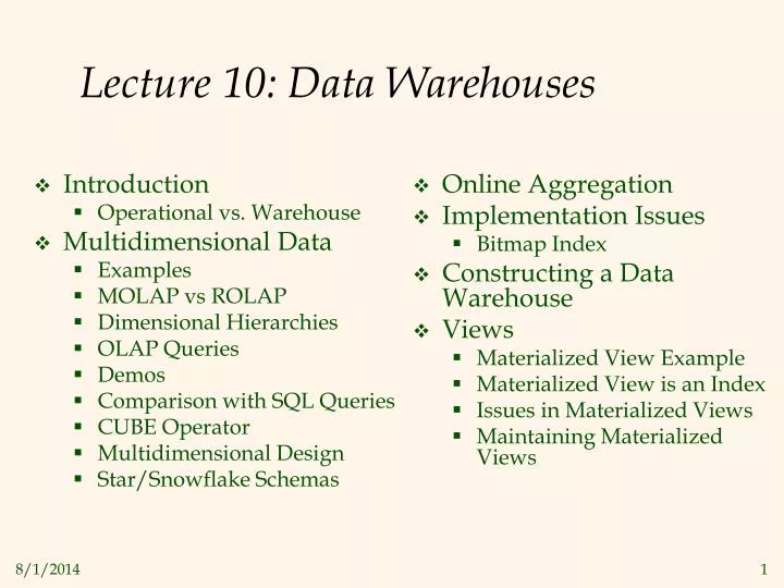
Lecture 10: Data Warehouses • Introduction • Operational vs. Warehouse • Multidimensional Data • Examples • MOLAP vs ROLAP • Dimensional Hierarchies • OLAP Queries • Demos • Comparison with SQL Queries • CUBE Operator • Multidimensional Design • Star/Snowflake Schemas • Online Aggregation • Implementation Issues • Bitmap Index • Constructing a Data Warehouse • Views • Materialized View Example • Materialized View is an Index • Issues in Materialized Views • Maintaining Materialized Views
Introduction • In the late 80s and early 90s, companies began to use their DBMSs for complex, interactive, exploratory analysis of historical data. • This was called Decision Support, and On-Line Analytic Processing (OLAP). • DS slowed down the operation of the company, called On-Line Transaction Processing (OLTP). • This led to the creation of Data Warehouses, separate from operational Databases.
Operational Warehouse General E-R Diagrams Multidimensional data model common Locks necessary No Locks necessary Crash recovery required Crash recovery optional Smaller volume of data Huge volume of data Need indexes designed to access small amounts of data Need indexes designed to access large volumes of data Operational vs Data Warehouse Requirements, ctd
OLAP Operational Data Data Warehousing EXTRACT TRANSFORM LOAD REFRESH • Integrated data spanning long time periods, often augmented with summary information. • Several terabytes to petabytes common. • Interactive response times expected for complex queries; ad-hoc updates uncommon. DATA WAREHOUSE Metadata Repository SUPPORTS DATA MINING
Multidimensional Data • In order to support OLAP, warehouse data is often structured multidimensionally, as measures and dimensions. • Measure: Numeric attribute, e.g. sales amount • Dimension: attribute categorizing the measure, e.g. product, store, date of sale. • The fact table is a foreign key for each dimension, plus an attribute for each measure. • There will also be a dimension table for each dimension. • On the next page, the fact tables are red, the dimension tables are green.
Examples of MultiDimensional Data • Purchase(ProductID, StoreID, DateID, Amt) • Product(ID, SKU, size, brand) • Store(ID, Address, Sales District, Region, Manager) • Date (ID, Week, Month, Holiday, Promotion) • Claims(ProvID, MembID, Procedure, DateID, Cost) • Providers(ID, Practice, Address, ZIP, City, State) • Members(ID, Contract, Name, Address) • Procedure (ID, Name, Type) • Telecomm (CustID, SalesRepID, ServiceID, DateID) • SalesRep(ID, Address, Sales District, Region, Manager) • Service(ID, Name, Category)
MOLAP vs ROLAP • Multidimensional data can be stored physically in a (disk-resident, persistent) array; called MOLAP systems. Alternatively, can store as a relation; called ROLAP systems. • The main relation, which relates dimensions to a measure, is called the fact table. Each dimension can have additional attributes and an associated dimension table. • E.g., Products(pid, locid, timeid, amt) • Fact tables are much larger than dimensional tables.
8 10 10 pid 11 12 13 30 20 50 25 8 15 1 2 3 timeid 25.2 Multidimensional Data Model timeid locid amt pid • Collection of numeric measures, which depend on a set of dimensions. • E.g., measure Amt, dimensions Product (key: pid), Location (locid), and Time (timeid). Slice locid=1 is shown: locid
Dimension Hierarchies • For each dimension, some of the attributes may be organized in a hierarchy: PRODUCT TIME LOCATION year category quarter state pname week city PID date ZIP
25.3 OLAP Queries • Influenced by SQL and by spreadsheets. • A common operation is to aggregate a measure over one or more dimensions. • Find total sales. • Find total sales for each city, or for each state. • Find top five products ranked by total sales. • Roll-up: Aggregating at different levels of a dimension hierarchy. • E.g., Given total sales by city, we can roll-up to get sales by state.
OLAP Queries • Drill-down: The inverse of roll-up. • E.g., Given total sales by state, can drill-down to get total sales by city. • E.g., Can also drill-down on different dimension to get total sales by product for each state. • Pivoting: Aggregation on selected dimensions. • E.g., Pivoting on State and Year yields this cross-tabulation: OR CA Total 63 81 144 2007 • Slicing and Dicing: Equality • and range selections on one • or more dimensions. 38 107 145 2008 75 35 110 2009 176 223 339 Total
Cognos Demo • Now we watch a demo of Cognos (bought by IBM) • Dimensions: Products…Margin ranges • Measure: Order value (sales) • First pivot from Product dimension to Margin Range • Notice how quickly the cube changes • Slice to Low Margin, pivot to Product and Company Region • Drill Down to High Tech, IDES AG • Now the guilty product is clear.
Tableau Demo • http://www.tableausoftware.com/products/tour2 • Note the many measures. • Pivot on sales, date (drill down to month), region as color. • Clear date, pivot on product and drill down on subcategory. • Change region from color to rows • Move profit into color • Change bars to circles • Pivot on dates (columns)
Comparison with SQL Queries • The cross-tabulation obtained by pivoting can also be computed using a collection of SQLqueries: SELECT T.year, L.state, SUM(S.amt) FROM Sales S, Times T, Locations L WHERE S.timeid=T.timeid AND S.locid=L.locid GROUP BY T.year, L.state SELECT T.year, SUM(S.amt) FROM Sales S, Times T WHERE S.timeid=T.timeid GROUP BY T.year SELECT L.state,SUM(S.amt) FROM Sales S, Location L WHERE S.locid=L.locid GROUP BY L.state
The CUBE Operator • Generalizing the previous example, if there are k dimensions, we have 2^k possible SQL GROUP BY queries that can be generated through pivoting on a subset of dimensions. • CUBE pid, locid, timeid BY SUM Sales • Equivalent to rolling up Sales on all eight subsets of the set {pid, locid, timeid}; each roll-up corresponds to an SQL query of the form: SELECT SUM(S.amt) FROM Sales S GROUP BY grouping-list Lots of work on optimizing the CUBE operator!
Example Multidimensional Design TIMES timeid date week month quarter year holiday_flag • This kind of schema is very common in OLAP applications • It is called a star schema • What is “wrong” with it? (Fact table) pid timeid locid amt SALES PRODUCTS LOCATIONS pid pname category price locid city state country
Star/Snowflake Schemas • Why normalize? • Space • Redundancy, anomalies • Why unnormalize? • Performance • Which is more important in D. Warehouses? • If normalized, it is a snowflake schema
Online Aggregation • Consider an aggregate query, e.g., finding the average sales by state. Can we provide the user with some information before the exact average is computed for all states? • Can show the current “running average” for each state as the computation proceeds. • Even better, if we use statistical techniques and sample tuples to aggregate instead of simply scanning the aggregated table, we can provide bounds such as “the average for Oregon is 2000±102 with 95% probability”. • Should also use nonblocking algorithms!
25.6 Implementation Issues • New indexing techniques: Bitmap indexes, Join indexes, array representations, compression, precomputation of aggregations, etc. • E.g., Bitmap index: sex custid name sex rating rating Bit-vector: 1 bit for each possible value. F M
Bitmap Indexes • Work when an attribute has few values, e.g. gender or rating • Advantage: Small enough to fit in memory • Many queries can be answered by bit-vector ops, e.g. females with rating = 3.
25.7 Constructing a D. Warehouse • Extract • Is the data in native format? • Clean • How many ways can you spell Mr.? • Errors, missing information • Transform • Fix semantic mismatches. • E.g. Last+first vs. Name • Load • Do it in parallel or else…. • Refresh • Both data and indexes
25.8,9 Views and Decision Support • In large databases, precomputation is necessary for decent response times • Examples: brain, google • Example: Precompute daily sums for the cube. • What can be derived from those precomputations? • These precomputed queries are called Materialized Views (SQL Server:Indexed views).
Materialized View Example CREATE VIEW DailySum(date, sumamt) AS SELECT date, SUM(amt) FROM Times Join Sales USING(timeid) GROUP BY date Mat.View Query SELECT week, SUM(amt) FROM Times Join Sales USING(timeid) Group By week Modified Query SELECT week, SUM(sumamt) FROM Times Join DailySum USING (week) GROUP BY week
Pros and Cons of Materialized Views • Pro: Modified query is a join of two small tables; original query is a join with one huge table. • Con: Materialized views take up space, need to be updated.
A Materialized View is an Index • Recall the definition of an index • Data structure that provides fast access to data • Table indexes were of the form {(value, pointer)}, perhaps at leaf level of a search structure. This is different. • Needs to be maintained as underlying tables change. • Ideally, we want incremental view maintenance algorithms.
What views should we materialize? • Remember the software that automatically chooses optimal index configurations? • The same software will choose optimal materialized views, given a workload and available space.
What about the optimizer? • Given a query and a set of materialized views, can we use the materialized views to answer the query? • This is tricky. Best reference is [348]
Refreshing Materialized Views • How often should we refresh the materialized view? • Many enterprises refresh warehouse data only weekly/nightly, so can afford to completely rebuild their materialized views. • Others want their warehouses to be current, so materialized views must be updated incrementally if possible. • Let's look at some simple examples.
25.10 Maintaining Materialized Views* • Incremental view maintenance • Defn: make changes in view that correspond to changes in the base tables • Example: V = SELECT a FROM R • How is V modified if r is inserted to R? • How is V modified if r is deleted from R?
Maintaining Materialized Views* • Consider V = R ⋈ S • How is V modified if r is inserted to R? • How is V modified if r is deleted from R? • Consider V = SELECT g,COUNT(*) FROM R GROUP BY g • How is V modified if r is inserted to R? • How is V modified if r is deleted from R • For more general cases, see [348]