Download
1 / 13
130 likes | 186 Vues
Learn about how mathematical representation ties to invariant ellipses in particle accelerator physics. Linear optics, emittance, and ellipse transformations explained.

E N D
Physics 417/517Introduction to ParticleAccelerator Physics G. A. Krafft Jefferson Lab Jefferson Lab Professor of Physics Old Dominion University
To summarize, this theorem gives a way to tie the mathematical representation of a unimodular matrix in terms of its α, β, and γ, and its phase advance, to the equations of the ellipses invariant under the matrix transformation. The equations of the invariant ellipses when properly normalized have precisely the same α, β, and γ as in the Twiss representation of the matrix, but varying c. Finally note that throughout this calculation c acts merely as a scale parameter for the ellipse. All ellipses similar to the starting ellipse, i.e., ellipses whose equations have the same α, β, and γ, but with different c, are also invariant under the action of M. Later, it will be shown that more generally is an invariant of the equations of transverse motion.
Applications to transverse beam optics When the motion of particles in transverse phase space is considered, linear optics provides a good first approximation of the transverse particle motion. Beams of particles are represented by ellipses in phase space (i.e. in the (x, x') space). To the extent that the transverse forces are linear in the deviation of the particles from some pre-defined central orbit, the motion may analyzed by applying ellipse transformation techniques. Transverse Optics Conventions: positions are measured in terms of length and angles are measured by radian measure. The area in phase space divided by π, ε, measured in m-rad, is called the emittance. In such applications, α has no units, β has units m/radian. Codes that calculate β, by widely accepted convention, drop the per radian when reporting results, it is implicit that the units for x' are radians.
Linear Transport Matrix Within a linear optics description of transverse particle motion, the particle transverse coordinates at a location s along the beam line are described by a vector If the differential equation giving the evolution of x is linear, one may define a linear transport matrix Ms',srelating the coordinates at s' to those at s by
From the definitions, the concatenation rule Ms'',s= Ms'',s'Ms',smust apply for all s' such that s < s'< s'' where the multiplication is the usual matrix multiplication. Pf: The equations of motion, linear in x and dx/ds, generate a motion with for all initial conditions (x(s), dx/ds(s)), thus Ms'',s= Ms'',s'Ms',s. Clearly Ms,s= I. As is shown next, the matrix Ms',s is in general a member of the unimodular subgroup of the general linear group.
Ellipse Transformations Generated by Hill’s Equation The equation governing the linear transverse dynamics in a particle accelerator, without acceleration, is Hill’s equation* Eqn. (2) The transformation matrix taking a solution through an infinitesimal distance ds is * Strictly speaking, Hill studied Eqn. (2) with periodic K. It was first applied to circular accelerators which had a periodicity given by the circumference of the machine. It is a now standard in the field of beam optics, to still refer to Eqn. 2 as Hill’s equation, even in cases, as in linear accelerators, where there is no periodicity.
Suppose we are given the phase space ellipse at location s, and we wish to calculate the ellipse parameters, after the motion generated by Hill’s equation, at the location s + ds Because, to order linear in ds, Det Ms+ds,s = 1, at all locations s, ε' = ε, and thus the phase space area of the ellipse after an infinitesimal displacement must equal the phase space area before the displacement. Because the transformation through a finite interval in s can be written as a series of infinitesimal displacement transformations, all of which preserve the phase space area of the transformed ellipse, we come to two important conclusions:
The phase space area is preserved after a finite integration of Hill’s equation to obtain Ms',s, the transport matrix which can be used to take an ellipse at s to an ellipse at s'. This conclusion holds generally for all s' and s. • Therefore Det Ms',s = 1for all s' and s, independent of the details of the functional form K(s). (If desired, these two conclusions may be verified more analytically by showing that may be derived directly from Hill’s equation.)
Evolution equations for the α, β functions The ellipse transformation formulas give, to order linear in ds So
Note that these two formulas are independent of the scale of the starting ellipse ε, and in theory may be integrated directly for β(s)and α(s)given the focusing function K(s). A somewhat easier approach to obtain β(s) is to recall that the maximum extent of an ellipse, xmax, is (εβ)1/2(s), and to solve the differential equation describing its evolution. The above equations may be combined to give the following non-linear equation for xmax(s) = w(s) = (εβ)1/2(s) Such a differential equation describing the evolution of the maximum extent of an ellipse being transformed is known as an envelope equation.
It should be noted, for consistency, that the same β(s) = w2(s)/ε is obtained if one starts integrating the ellipse evolution equation from a different, but similar, starting ellipse. That this is so is an exercise. The envelope equation may be solved with the correct boundary conditions, to obtain the β-function. α may then be obtained from the derivative of β, and γ by the usual normalization formula. Types of boundary conditions: Class I—periodic boundary conditions suitable for circular machines or periodic focusing lattices, Class II—initial condition boundary conditions suitable for linacs or recirculating machines.
Solution to Hill’s Equation inAmplitude-Phase form To get a more general expression for the phase advance, consider in more detail the single particle solutions to Hill’s equation From the theory of linear ODEs, the general solution of Hill’s equation can be written as the sum of the two linearly independent pseudo-harmonic functions where
are two particular solutions to Hill’s equation, provided that Eqns. (3) and where A, B, and c are constants (in s) That specific solution with boundary conditions x(s1) = x1 and dx/ds (s1) = x'1 has