Download
1 / 34
350 likes | 466 Vues
CUFSM Advanced Functions. CUFSM 2.5. Boundary conditions Constraints Springs Multiple materials Orthotropic Material. Boundary conditions. Longitudinal boundary conditions (fixity) can be set in the finite strip model Modeling classic problems requires using this feature

E N D
CUFSM Advanced Functions CUFSM2.5 • Boundary conditions • Constraints • Springs • Multiple materials • Orthotropic Material
Boundary conditions • Longitudinal boundary conditions (fixity) can be set in the finite strip model • Modeling classic problems requires using this feature • simply supported plate • fixed plate • Special cases may exist where artificial boundary conditions are added in an analysis to examine a particular buckling mode in exclusion of other modes (see Advanced Ideas for more on this) • Symmetry and anti-symmetry conditions may be modeled by modifying the boundary conditions
Boundary conditions continued • How to • Simply supported plate example • Fixed-free plate example • Flange only model • Symmetry model on a hat in bending example
How to (boundary conditions) These columns of ones set the boundary conditions for the model. A 1 implies that the degree of freedom is free along its longitudinal edge. All models are simply supported at the ends due to the choice of shape function in the finite strip method. For models of members these always remain 1, however if longitudinal restraint should be modeled then the appropriate degree of freedom (direction) should be changed from a 1 to a 0. z q x y
Simply supported plate (boundary conditions) Simply supported plate in pure compression Plate is 10 in. wide and t = 0.10 in., material is steel. The x and z degree of freedom at node 1 have been supported by changing the appropriate 1’s to 0’s. The z degree of freedom at node 5 has been supported by changing the appropriate 1 to 0. Green boxes appear at 1 and 5 to indicate some boundary conditions have been changed at this node.
Simply supported plate (boundary conditions) Input reference stress is 1.0 ksi. So in this case the load factor is equal to the buckling stress in ksi, i.e., 10.67 ksi. versus 10.66 ksi by hand.
Fixed-free plate (boundary conditions) Fixed-free plate in pure compression Plate is 10 in. wide and t = 0.10 in., material is steel. The x, z and q (q) degree of freedom at node 1 have been supported by changing the appropriate 1’s to 0’s. Green boxes appear at 1 to indicate some boundary conditions have been changed at this node.
Fixed-free plate (boundary conditions) Input reference stress is 1.0 ksi. So in this case the load factor is equal to the buckling stress in ksi, i.e., 3.42 ksi. versus 3.40 ksi by hand.
Flange only model (boundary conditions) Isolated flange in pure compression Plate is 10 in. wide and t = 0.10 in., material is steel.Lip is 2 in. long and the same material and thickness The x, z and q (q) degree of freedom at node 1 have been supported by changing the appropriate 1’s to 0’s. So, the left end is “built-in” or “fixed”.
Flange only model (boundary conditions) fixed Adding the lip stiffener increases the buckling stress significantly. Adding the lip stiffeners introduces the possibility of two modes, one local, one distortional. Local Distortional
Symmetry model on a hat in bending (boundary conditions) Hat in bending - full model The hat is 2 x 4 x 10 in. Pure bending is applied as the reference load. The reference compressive stress for the top flange is 1.0 ksi which results in -1.75 tension for the bottom flange
Symmetry model on a hat in bending (boundary conditions) Hat in bending - half model The hat is 2 x 4 x 10 in. Pure bending is applied as the reference load. The reference compressive stress for the top flange is 1.0 ksi which results in -1.75 tension for the bottom flange. Symmetry conditions are enforced at mid-width of the top flange, note the degrees of freedom changed to 0 at node 11 in the Nodes list to the left.
Symmetry model on a hat in bending (boundary conditions) full model local buckling stress in compression = 15.11 ksi
Symmetry model on a hat in bending (boundary conditions) half model using symmetry local buckling stress in compression = 15.11 ksi
Constraints • You may write an equation constraint: this enforces the deflection (rotation) of one node to be a function of the deflection (rotation) of a second node. • Modeling external attachments may be aided by using this feature • an external bar that forces two nodes to have the same translation but leaves them otherwise free • a brace connecting two members (you can model multiple members in CUFSM) • Special cases may exist where artificial equation constraints are added in an analysis to examine a particular buckling mode in exclusion of other modes (see Advanced Ideas for more on this)
Constraints continued • How to • Connected lips in a member • Multiple connected members
How to (constraints) Equation Constraints are determined by defining the degree of freedom of 1 node in terms of another. For example, the expression below in Constraints says At node 1, set degree of freedom 2 equal to 1.0 times node 10, degree of freedom 2: w1=1.0w10 You can enter as many constraints as you like, but once you use a degree of freedom on the left hand side of the equation it is eliminated and can not be used again. Symbols appear on the nodes that you have written constraint equations on, as shown in this plot for nodes 1 and nodes 10.
Connected lips in a member (constraints) Constraints example 1 Use the default member Change the loading to pure compression Constrain the ends of the lips, nodes 1 and 10 to have the same vertical displacement Compare against analysis which does not have this constraint.
Connected lips in a member (constraints) Loading is pure compression with a reference stress of 1.0, the two results show the influence of the constraint on the solution. The two lips have the same vertical displacement. Anti-symmetric distortional buckling results. distortional with the constraints on the lips typical distortional buckling local is the same
Multiple connected members (constraints) Multiple Member Equation Constraint Example Two members are placed toe-to-toe. Geometry is the default Cee section in CUFSM. The loading is pure compression. In this example only the top lips are connected, say for example because of an unusual access situation. Equation constraints are written, as shown below to force that x, z and q of nodes 10 and 20 are identical.
Multiple connected members (constraints) Local buckling is not affected by the constraint, but distortional buckling and long wavelength buckling is… top lips are connected. This has an influence on distortional buckling, as shown. weak-axis flexural buckling occurs in the model with the lips attached at the top. local and distortional buckling for a single member. flexural-torsional buckling occurs in the single isolated member
Springs • External springs may be attached to any node. • Modeling continuous restraint may use this feature • Continuous sheeting attached to a bending member might be considered as springs • Sheathing or other materials attached to compression members might be considered as springs • Springs may be modeled as a constant value, or as varying with the length of the model (i.e. a foundation)
Springs • How to • Sheeting attached to a purlin • Spring verification problem
How to (springs) Springs are determined by defining the node where a spring occurs, what degree of freedom the spring acts in, the stiffness of the spring, and whether or not the spring is a constant value (e.g. force/length) or a foundation spring (e.g. (force/length)/length). Constant springs use kflag=0, foundations use kflag=1. You can enter as many springs as you like. The springs always go to “ground”. Therefore they cannot be used to connect two members. Springs appear in the picture of your model once you define them. Springs are modeled as providing a continuous contribution along the length.
Sheeting attached to a purlin (springs) Purlin with a sheeting “spring” example Use the LGSI Z 12 x 2.5 14g model from Tutorial 3 The applied bending stress is restrained bending about the geometric axis with fy=50 ksi. (first yield is in tension in this model as the flange widths are slightly different sizes) Assume a spring of k = 1.0 (kip/in.)/in. exists in the vertical direction at mid-width of the compression flange. (Ignore, in this case, rotational stiffness contributions from the sheeting, etc.) See Springs below for the definition of the vertical spring.
Sheeting attached to a purlin (springs) The buckling curve below shows the results of an analysis without the springs (1) and analysis with the spring (2). Note that the spring has greatly increased the distortional buckling stress. The buckling mode to the left shows distortional buckling with the spring in place. Note, the “star” denotes the existence of the spring in the model. Example for demonstrative purposes only - actual sheeting may have much lower stiffness, and other factors may be considered in the analysis.
Multiple materials • Multiple materials may be used in a single CUFSM model • Explicitly modeling attachments that are of different materials may use this feature • Some unusual geometry changes may be modeled by changing the material properties
explicit sheathing modeling 0.25 in. thick sheet E=1/10Esteel, see mat# 200 perfect connection at mid-width between stud and sheathing done by constraints. Toe-to-toe studs with 1-sided Sheathing Use a pair of the default CUFSM Cee sections and connect them to a 0.25 in. sheathing on one flange only. The sheathing should have E=1/10Esteel Note, the use of a second material and the constraints that are added to model the connection.
explicit sheathing modeling Toe-to-toe studs with 1-sided Sheathing Material numbers are shown using the material# check-off in the plotting section. The loading is pure compression on the studs, and no stress on the sheathing.
explicit sheathing modeling Local buckling is not affected by the sheathing, but distortional buckling and long wavelength buckling is… weak-axis flexural buckling occurs in the model with the sheathing local and distortional buckling for a single member. flexural-torsional buckling occurs in a single isolated member
Orthotropic Material • Orthotropic materials may be used in CUFSM • Plastics, composites, or highly worked metals may benefit from using this feature
1/2 G, SS Plate Orthotropic Material Example Simply supported plate where Gxy is 1/2Gisotropic Low G modulus are typical concerns with some modern plastics and other materials. Also, some sheathing materials may be modeled orthotropically.
1/2 G, SS Plate CUFSM2.5 vs. 8.80 ksi when Gxy = 1/2Gisotropic