Download
1 / 85
930 likes | 1.2k Vues
Flexible Coding for 802.11n MIMO Systems. Keith Chugg and Paul Gray TrellisWare Technologies Bob Ward SciCom Inc. kchugg@trellisware.com (with support provided by UCLA’s UnWiReD Lab.). Overview. TrellisWare’s Flexible-Low Density Parity Check (F-LDPC) Codes

E N D
Flexible Coding for 802.11n MIMO Systems Keith Chugg and Paul Gray TrellisWare Technologies Bob Ward SciCom Inc. kchugg@trellisware.com (with support provided by UCLA’s UnWiReD Lab.) Keith Chugg, et al, TrellisWare Technologies
Overview • TrellisWare’s Flexible-Low Density Parity Check (F-LDPC) Codes • FEC Requirements for IEEE 802.11n • Introduction to F-LDPC Codes • F-LDPC Turbo/LDPC dual interpretation • Example Applications of F-LDPC Codes to the IEEE 802.11n PHY Layer • SVD-based MIMO-OFDM with Adaptive Rate Allocation • MMSE-SIC V-BLAST MIMO-OFDM • Conclusions Keith Chugg, et al, TrellisWare Technologies
FEC Requirements for IEEE 802.11n • Frame size flexibility • Packets from MAC can be any number of bytes • Packets may be only a few bytes in length • Byte-length granularity in packet sizes rather than OFDM symbol • Code rate flexibility • Need fine rate control to make efficient use of the available capacity • Good performance • Need codes that can operate close to theory for finite block size and constellation constraint • High Speed • Need decoders that can operate up to 300-500 Mbps • Low Complexity • Need to do all this without being excessively complex • Proven Technology • Existing high-speed hardware implementations Keith Chugg, et al, TrellisWare Technologies
Benefits of Modern FEC Flexibility for 802.11n • Flexibility in code rate and modulation • Large range of spectral efficiencies (bps/Hz) with fine resolution • Maximize the data rate for the current channel conditions • Minimizes need for pad bits • Flexibility in the Block Size • Essential for the MAC • Block size selection on-the-fly allows one to optimally meet latency requirements • “Future Proof” • High FEC flexibility will support virtually any evolution of the standard and unforeseen operational scenarios • Can alter FEC block length to account for changes in the latency budget (hardware, software implementation technology) Keith Chugg, et al, TrellisWare Technologies
F-LDPC Encoder P/S (2:1) S/P (1:J) input bits parity bits SPC Outer Code Inner Code … I J bits wide systematic bits TrellisWare’s F-LDPC Codes • A Flexible-Low Density Parity Check Code (F-LDPC) • Systematic code overall • Concatenation of the following elements: • Outer code: 2-state rate ½ non-recursive convolutional code • Flexible algorithmic interleaver • Single Parity Check (SPC) code • Inner Code: 2-state rate 1 recursive convolutional code Keith Chugg, et al, TrellisWare Technologies
TrellisWare’s F-LDPC Codes (2) • Use of 2-state constituent codes means very low decoder complexity • Outer code polynomials: (1+D, 1+D) • Inner code polynomial: (1/(1+D)) [accumulator] • Outer code uses tail-biting termination • Inner code is not terminated • For K-bit frames the interleaver is fixed at 2K bits, regardless of rate. • Any good algorithmic interleaver will give frame size programmability down to bit level • SPC forms single-parity check of J bits. • Different code rates are achieved by only varying J • Code rate = J/(J+2) • Inner code runs at 1/J fraction of speed of outer code Keith Chugg, et al, TrellisWare Technologies
F-LDPC Features • Unparalleled flexibility without complexity penalty • Input Block Sizes: 3 bytes to 1000 bytes in single byte increments • Code Rate: ½ to 32/33 with virtually any rate in between • Uniformly good performance over these modes • ~< 1 db of SNR from random coding bounds (best point designs are 0.5 dB) • Low complexity traits of LDPC codes • Similar edge complexity • Lower memory requirements and simpler memory design and access • Proven high-speed hardware implementation • 300 Mbps single FPGA prototype • F-LDPC code is simplification of TrellisWare’s FlexiCode ASIC design • Options for architectures associated with LDPC decoders and Turbo decoders Keith Chugg, et al, TrellisWare Technologies
F-LDPC Alternative Interpretations • Proposed code can be viewed as either • Concatenation of two-state convolutional codes with a single-parity check (SPC) block code • Punctured irregular-LDPC (IR-LDPC) • IR-LDPC • Proposed code can be decoded using • Forward-backward algorithm (BCJR) type SISO decoders (typically associated with concatenated convolutional codes) • Parallel “check node” and “variable node” processors (typically associated with LDPC codes) Keith Chugg, et al, TrellisWare Technologies
F-LDPC Alternative Interpretations (2) • Performance is comparable to good IR-LDPC codes • Near best performance of best known codes over wide range of block sizes and code rates • Decoding complexity (measured by operation counts) is very low • Similar to that of the IR-LDPC used in DVB-S2 • Significantly less than that of an 8-state PCCC (e.g., 3GPP) • Both LDPC and “turbo” architectures can be used • Third parties with good solutions for concatenated convolutional codes and LDPC codes can apply their technology • Yields high degree of freedom for trade-off between parallelism, memory architectures, etc. Keith Chugg, et al, TrellisWare Technologies
F-LDPC as Concatenated CCs Encoder P/S (2:1) S/P (1:J) K input bits V=(2K)/J parity bits SPC 1+D 1/(1+D) … I 1+D Rate=J/(J+2) J bits wide “zig-zag” code K systematic bits Decoder (standard rules of iterative decoding) Channel Metrics (LLRs) for parity bits > < 0 Outer SISO I-1 SPC SISO Inner SISO … Hard decisions I J bits wide “zig-zag” SISO Channel Metrics (LLRs) for systematic bits Note: activation begins with outer code Keith Chugg, et al, TrellisWare Technologies
F-LDPC as Punctured IR-LDPC Recall: Encoder PTc e c Tc SPC 1+D p 1/(1+D) … I b 1+D (K x 1) (K x 1) (2K x 1) J bits wide “zig-zag” code b c = Gb e = JPTc e + Sp = 0 G: generator of outer (1+D) code (K x K) S: “staircase” accumulator block (V x V) T: repeat outer code bit twice (2K x K) P: permutation of interleaver (2K x 2K) J: SPC mapping (V x 2K ) p S JPT 0 V c = 0 0 I G K b V K K Low Density Parity Check: Hc’ = 0 Keith Chugg, et al, TrellisWare Technologies
1 0 0 … 0 0 1 1 1 0 0 … 0 0 0 0 1 1 0 0 … 0 0 0 0 1 1 0 0 … 0 0 0 0 1 1 0 … 0 0 0 … 0 0 1 1 0 0 0 0 … 0 0 1 1 1 0 0 … 0 0 0 1 0 0 0 … 0 0 0 0 1 0 0 0 … 0 0 0 1 0 0 0 0 … 0 0 0 1 0 0 0 … 0 0 0 1 0 0 0 … 0 0 0 0 1 0 0 … 0 0 0 0 1 0 0 … 0 0 0 … 0 0 0 1 0 0 0 0 … 0 0 1 0 0 0 … 0 0 0 0 1 0 0 0 … 0 0 0 1 J 0 1 1 … 1 1 1 … 1 1 1 … 1 0 1 1 … 1 … 1 1 … 1 F-LDPC as Punctured IR-LDPC (2) 1 0 0 … 0 0 0 1 1 0 0 … 0 0 0 0 1 1 0 0 … 0 0 0 0 1 1 0 0 … 0 0 0 0 1 1 0 … 0 0 0 … 0 0 1 1 0 0 0 0 … 0 0 1 1 0 0 0 0 … 1 0 0 0 0 0 1 … 0 0 0 1 0 0 0 0 … 0 0 0 0 … 1 0 0 0 0 0 1 0 … 0 0 0 0 G = S = P = T = (pseudo-random permutation matrix) (2K x 2K) (K x K) (V x V) This element is 1 if outer code is tail-bit; 0 if unterminated This element is 1 if outer code is tail-bit; 0 if unterminated (2K x K) S JPT 0 J = H = 0 I G (V x 2K) Keith Chugg, et al, TrellisWare Technologies
F-LDPC as Punctured IR-LDPC (3) Inner (zig-zag) code Present if inner code it tail-bit … J J J J J I/I-1 2 2 2 2 2 … Present if outer code it tail-bit Outer code Keith Chugg, et al, TrellisWare Technologies
3 3 3 3 3 … F-LDPC as Punctured IR-LDPC (4) K check nodes (from outer code); (dc=3) V=(2K/J) check nodes (from inner code); (dc=J+2) … … 3 3 3 3 J+2 J+2 J+2 3 J+2 J+2 Structured Permutation 2 2 2 2 2 2 2 2 2 2 … … p:V=(2K/J) parity bits (dv=2) b: K Systematic Bits (dv=2) c: K (hidden) bits (dv=3) Note: this assumes inner and outer codes are tail-bit. If not, there will be a small difference as implied in the previous slides Keith Chugg, et al, TrellisWare Technologies
F-LDPC as Punctured IR-LDPC (5) Example of degree distribution for various code rates • Complexity is roughly measured by number of edges in the parity check graph • F-LDPC has edge complexity slightly less than the DVB-S2 IR-LDPC code Keith Chugg, et al, TrellisWare Technologies
F-LDPC as Punctured IR-LDPC (6) • Decoder Activation schedules • “Standard LDPC”: parallel variable-node, parallel check node • Number of internal messages stored = number of edges (~7K) • “Piecewise Parallel (green-red-blue)” schedule • Number of internal messages stored (~2K) • “Standard Concatenated Convolutional Code” schedule • Same as discussed when interpreting F-LDPC as CCC • Number of internal messages stored (~2K) • Piecewise Parallel and Standard CCC exploit structure of the punctured IR-LDPC permutation Keith Chugg, et al, TrellisWare Technologies
3 3 3 3 3 … F-LDPC as Punctured IR-LDPC (7) … … 3 3 3 3 J+2 J+2 J+2 3 J+2 J+2 I/I-1 2 2 2 2 2 2 2 2 2 2 … … • Structure of permutation enables potential memory savings and different high-speed decoding architectures Keith Chugg, et al, TrellisWare Technologies
F-LDPC as Punctured IR-LDPC (8) Standard LDPC schedule (~7K internal messages stored) 2 2 2 2 2 2 1 1 1 1 1 1 Piecewise Parallel (green-red-blue) schedule (~2K internal messages stored) 2 8 7 3 6 4 5 1 Standard CCC schedule (Outer SISO -> Inner SISO; ~2K messages) Outer SISO Inner SISO Keith Chugg, et al, TrellisWare Technologies
F-LDPC as Punctured IR-LDPC (9) • Schedule properties • All are examples of the same standard iterative message-passing decoding rules with different activation schedules • Each have the same computational complexity per iteration • Iteration convergence, degree of parallelism,memory needs, etc. vary with schedule Keith Chugg, et al, TrellisWare Technologies
F-LDPC as IR-LDPC • Possible to eliminate hidden variables • Formulates the F-LDPC as in a standard IR-LDPC format • i.e., N variable nodes, V=(N-K) check nodes p S JPT 0 V p V c = 0 = S JPTG 0 I G V K b b K V K K K V Keith Chugg, et al, TrellisWare Technologies
F-LDPC as IR-LDPC (2) • Degree distribution • For high-spread interleaver and K>>J • V variable nodes with dv=2 • K variable nodes with dv=4 • All checks have dc=2J+2 • Example: r=1/2: 50% dv=2, 50% dv=4, dc=6 • This form has many four-cycles • Modified schedule or H-matrix transformations likely required for good performance based on this graphical model Keith Chugg, et al, TrellisWare Technologies
Example Applications of F-LDPC Codes to the IEEE 802.11n PHY Layer Keith Chugg, et al, TrellisWare Technologies
11n Encoder output symbols P/S (2:1) S/P (1:M) systematic bits input bits F-LDPC Encoder Coded Bit Interleaver Flexible Mapper I … Puncture Q parity bits F-LDPC Applied to IEEE 802.11n • A single, flexible encoder that is suitable for use in a variety of MIMO-OFDM systems • F-LDPC encoder is coupled with a simple puncture circuit for fine rate control, a bit channel interleaver, and a flexible mapper of QAM symbols to the MIMO-OFDM subcarrier frequencies • Code rate and modulation profile can be tuned to maximize throughput Keith Chugg, et al, TrellisWare Technologies
F-LDPC Applied to IEEE 802.11n (2) • F-LDPC Encoder • 3-1024 input bytes, in single byte increments (negligible performance gains above 1Kbytes) • Block size is programmable on the fly and can be used to meet latency requirements • 5 Coarse rates of r = 1/2, 2/3, 4/5, 8/9, and 16/17 • Fine rate control with a simple algorithm • Provides fine resolution – especially for code rates between ½ and 2/3 • 9 Fine rates of p = 16/16, 15/16,…., 8/16 • Overall rate of r/(r+p(1-r)), with r=J/(J+2) • 45 code rates from 1/2 to 32/33 • Fine rate control means that pad bits can be minimized • Coded Bit Interleaver • Bit interleaving of a single code word • A simple relative prime interleaver is used here (the size of this interleaver must be very flexible) • Flexible Mapper • 5 modulations of BPSK, QPSK, 16QAM, 64QAM, and 256QAM (more possible) • Gray mapping • Bit-loading is easily supported Keith Chugg, et al, TrellisWare Technologies
Uniformly Good Performance • PER vs. SNR curves are shown for a range of code rates and modulation orders • Min-sum decoding (“log-max-APP”) • 1% PER can be achieved from -2 dB to 27 dB SNR in approximately 0.25 steps • Bandwidth efficiency is shown against SNR required to achieve a PER of 1% • Full range of code rate, modulation types, and frame sizes (from 128 to 8000 information bits) • Performance is compared with finite block size bound and capacity • Generally within 1 dB of finite block size bound • Higher order modulation performance could be improved by iterating the soft-demapper (more complex though) • Demonstrates the fine code rate granularity possible Keith Chugg, et al, TrellisWare Technologies
AWGN Perf.: Varying Rate & Modn. 1 0.1 PER 0.01 0.001 0 5 10 15 20 25 30 SNR (dB) ~0.25 dB Rate 1/2 BPSK – 32/33 256QAM Keith Chugg, et al, TrellisWare Technologies
AWGN Perf.: Bandwidth Efficiency 8 128 bits 256 bits 7 512 bits 1024 bits 2048 bits 6 8000 bits 5 Bandwidth Efficiency (info bits/symbol) 4 3 2 1 Rate 1/2 - 32/33 0 -5 0 5 10 15 20 25 30 Required SNR for 1% PER (dB) 256QAM 64QAM 16QAM QPSK BPSK Keith Chugg, et al, TrellisWare Technologies
AWGN Perf.:Comparison with Bound 9 BPSK QPSK 8 16QAM 64QAM 7 6 5 Bandwidth Efficiency (info bits/symbol) 4 3 2 1 0 -5 0 5 10 15 20 25 30 Required SNR for 1% PER (dB) 256QAM BPSK Bound QPSK Bound 16QAM Bound 64QAM Bound 256QAM Bound log2(1 + SNR) All 8000 info bits Keith Chugg, et al, TrellisWare Technologies
Frame Size Flexibility • Coding and modulation is fixed at rate 4/5 16QAM • PER vs. SNR curves are shown for a range of frame sizes from 8 to 1000 bytes • SNR required to achieve a PER of 1% is shown against frame size • Both automated search and hand tuned interleaver parameters are shown. It is expected that performance matching that of the hand tuned parameters can achieved everywhere • The finite block size performance bound is also plotted, showing that the automated search parameters are within 1 dB of this bound, and the hand tuned parameters are with 0.75 dB Keith Chugg, et al, TrellisWare Technologies
AWGN Perf.: Frame Size Flexibility 1 0.1 PER 0.01 1000 bytes 8 bytes Frame Size 0.001 10.5 11 11.5 12 12.5 13 13.5 14 SNR (dB) All 4/5 16QAM Keith Chugg, et al, TrellisWare Technologies
AWGN Perf.: Frame Size Flexibility (2) 13.5 Automated search parameters 13 12.5 12 Required SNR for 1% PER (dB) 11.5 11 10.5 10 0 1000 2000 3000 4000 5000 6000 7000 8000 Frame Size (bits) Hand tuned parameters Finite block bound Modulation constrained capacity Keith Chugg, et al, TrellisWare Technologies
Early Stopping • F-LDPC codes can use early-stopping to reduce the average number of iterations and decreasing complexity for a given data throughput • Performance with early stopping is almost as good as that with 32 iterations • Flow control algorithm active with early stopping results • 50% larger input buffer is assumed • Average iterations as a function of required SNR for a 1% PER • With early stopping the average number of iterations is less than 12 • Average number of iterations reduces as the code rate increases • 32 iteration performance with an average of less than 12 iterations Keith Chugg, et al, TrellisWare Technologies
AWGN Perf.: Early Stopping 8 BPSK 32 its QPSK 32 its 7 16QAM 32 its 64QAM 32 its 256QAM 32 its 6 BPSK Early Stopping QPSK Early Stopping 5 16QAM Early Stopping 64QAM Early Stopping Bandwidth Efficiency (info bits/symbol) 4 256QAM Early Stopping 3 2 1 0 -5 0 5 10 15 20 25 30 Required SNR for 1% PER (dB) Keith Chugg, et al, TrellisWare Technologies
Higher Code Rates Converge Faster Keith Chugg, et al, TrellisWare Technologies
Decoder Throughput • Structure of the code lends itself to low complexity, high speed decoding • We have used a baseline high speed architecture with a nominal degree of parallelism of P=1 • P=n throughput is n times higher, and complexity is n times greater • Plots for both throughput normalized to the system clock (bps per clk) and actual throughput with a number of system clock assumptions • Existing P=8 FPGA prototype • System clock of 100 MHz • Throughput is 300 Mbps @ 10 iterations • Xilinx XC2V8000 Keith Chugg, et al, TrellisWare Technologies
Decoder Throughput – Bps/Clock 10 P = 1 P = 2 P = 4 P = 8 8 6 Decoder Throughput (bps per clock) 4 2 0 5 10 15 20 25 30 Iterations Keith Chugg, et al, TrellisWare Technologies
Decoder Throughput – P=4 and P=8 600 P=4 f=100 MHz P=8 f=100 MHz P=4 f=150 MHz 500 P=8 f=150 MHz P=4 f=200 MHz P=8 f=200 MHz 400 P=4 f=250 MHz P=8 f=250 MHz P=4 f=300 MHz Decoder Throughput (Mbps) 300 P=8 f=300 MHz FPGA Prototype: 300 Mbps 100 MHz Xilinx XC2V8000 200 100 10 iterations 0 5 10 15 20 25 30 Iterations Keith Chugg, et al, TrellisWare Technologies
Decoder Latency • Decoder latency needs to be < ~6 μs • Last bit in to first bit out • This can be achieved by a P=8 decoder with a 200 MHz clock • 12 iterations • < ~2048 bit code words • With large MAC packets just ensure that final code word of packet is <2048 bits • As technology improves (higher clock or larger P) this minimum code word size can be increased Keith Chugg, et al, TrellisWare Technologies
20 P=4 f=100 MHz P=8 f=100 MHz P=4 f=150 MHz P=8 f=150 MHz P=4 f=200 MHz 15 P=8 f=200 MHz P=4 f=250 MHz P=8 f=250 MHz P=4 f=300 MHz Decoder Latency (us) 10 P=8 f=300 MHz 5 0 0 1000 2000 3000 4000 5000 6000 7000 8000 Block Size Decoder Latency (12 iterations) 6 μs Keith Chugg, et al, TrellisWare Technologies
F-LDPC High Speed Implementation • Proven Technology • FPGA implementations of F-LDPC • 300 Mbps @ 10 iterations with 100 MHz clock • Xilinx XC2V8000 • ASIC implementation of FlexiCode • A version of the F-LPDC with 4-state codes • More complex than F-LDPC with more features • BER of 10-10 in all modes • 196 Mbps @ 10 iterations with 125 MHz clock • 0.18 μm standard cell process Keith Chugg, et al, TrellisWare Technologies
F-LDPC High Speed Implementation(2) Keith Chugg, et al, TrellisWare Technologies
F-LDPC Examples for IEEE 802.11n • SVD-based MIMO-OFDM Example • Assume perfect CSI at the Tx and Rx • Adaptive power and rate allocation via a simple code-driven algorithm • Greater than 300 Mbps demonstrated • V-BLAST Example • No Tx-CSI • MMSE interference suppression • Independent application of TW’s F-LDPC code DLL by UCLA’s UnWiReD Lab. (Prof. Mike Fitz) • Desired Packet error rates demonstrated Keith Chugg, et al, TrellisWare Technologies
SVD-based Example 802.11n model Keith Chugg, et al, TrellisWare Technologies
SVD-based Example: Power Allocation • Approaches Considered • Space-Frequency Water-Filling (SFWF) • “Constant Power Water-Filling (CPWF)” in Space and Frequency (Yu & Cioffi, 2003) • Select a subset of subchannels to use and allocate power equally among these active subchannels • “Code Driven CPWF” in Space and Frequency • Compute the subchannel SNR assuming a constant power allocation across all subchannels • If this is less than the minimum SNR supported by the FEC, do not use this subchannel (e.g., -2 dB for 8000 bit input blocks). • Allocate power equally across subchannels used Keith Chugg, et al, TrellisWare Technologies
SVD-based Example: Power Allocation (2) Keith Chugg, et al, TrellisWare Technologies
SVD-based Example: Rate Allocation • Given a set of subchannels with equal power assignments and known gain distribution • 1) Select modulation order (M) by FEC’s performance • 2) Compute AWGN channel capacity with Gaussian signals, with SNR degraded to account for finite block size, non-Gaussian signals, and imperfect FEC (=C) • 3) Compute channel bits carried by offered subchannels with given modulation assignments (=B) • 4) Select FEC code rate as r=C/B • Sets target information rate at the capacity plus the small code degradation • This requires a very flexible, uniformly good FEC solution Keith Chugg, et al, TrellisWare Technologies
SVD-based Example: Rate Allocation (2) • K=8000 Input Bits • 1) Subchannel i: use SNR(i) to set M(i) • SNR(i) <1.5 dB => BPSK • 1.5 dB<SNR(i) <6.6 dB => QPSK • 6.6 dB<SNR(i) <13 dB => 16QAM • 13 dB<SNR(i) <20 dB => 64QAM • SNR(i) >20 dB => 256QAM • 2) FEC is ~2.9 dB from AWGN capacity • C=Σ(log2(1+SNR(i)*0.52)) • 3) Channel bits available • B= Σ (log2(M(i)) • 4) r= B/C Keith Chugg, et al, TrellisWare Technologies
SVD-based Example: Performance • Channel was the IST project IST-2000-30148 I-METRA Matlab model (NLOS) • The following plots assume a 802.11a/g OFDM structure: • 64 sub-carriers/20 MHz sampling rate • Same sub-carrier structure • 48 sub-carriers for data, 4 sub-carriers for pilot • “DC” sub-carrier empty, 11 sub-carriers for guard band • 3.2 µs symbol, 800 ns cyclic prefix • Both 8000 bit (best performance) and 2048 bit (low latency) • Rate and power allocation as described previously • Tests run with nominal SNR into the rate adaptation algorithm of 0, 5, 10, 15, 20, and 25 dB • Perfect synchronization and perfect CSI • Early stopping + buffer overflow protection enabled Keith Chugg, et al, TrellisWare Technologies
SVD –based Example: 1x1 Channel B Keith Chugg, et al, TrellisWare Technologies
SVD –based Example: 2x2 Channel B Keith Chugg, et al, TrellisWare Technologies